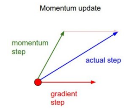
动量(momentum)更新是梯度下降的一种优化方法,它能够加快损失函数收敛速度(converge rate)
标准梯度下降 标准梯度下降公式如下:
\[ w_{t} = w_{t-1} - lr\triangledown f(w_{t-1}) \]
\(lr\) 是固定值,表示步长,所以在假设梯度不变的情况下,每次更新沿着参数的负梯度方向前进固定步长
经典动量 经典动量(classical momentum,简称CM)公式如下
\[ v_{t} = \mu v_{t-1} - lr\triangledown f(w_{t-1}) \\ w_{t} = w_{t-1} + v_{t} \]
\(v\) 表示速度,初始化为0
\(\mu\) 表示动量因子(momentum coefficient),大小为\([0,1]\) ,表示当前权重变化受过去累计梯度的影响
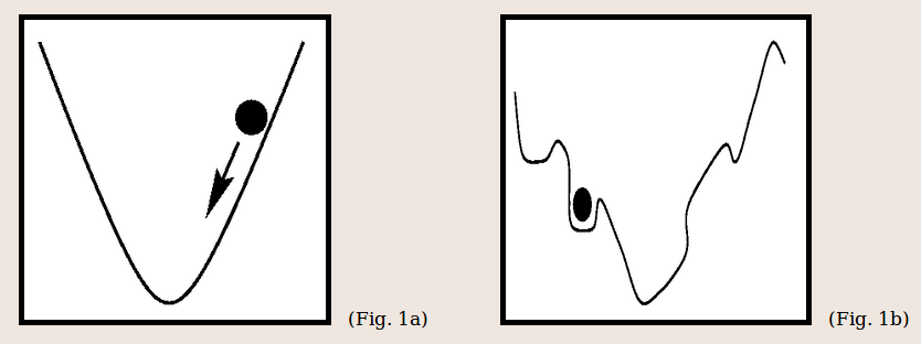
物理视角 从物理视角看损失函数收敛问题,将损失值看成丘陵地形(hilly terrain)的高度。对于初始化权重(\(w\) )而言,它相当于设置在某个位置的初始速度(initial velocity )为0的粒子(particle)。所以优化过程(optimization process)等同于模拟粒子在陆地上滚动的过程
驱动粒子滚动的力就是势能负梯度(\(F = -\triangledown U\) ),对于势能(\(U=mgh\) )而言,它和高度(\(h\) )呈正相关(\(U\propto h\) )
在标准梯度下降中,势能梯度直接用于修改粒子滚动的距离
在经典动量中,将力作用于粒子的速度和方向(\(F=ma\) ),再间接影响滚动的距离
当力作用方向和累计速度方向一致时,就能够加快粒子滚动速度;与此同时,当力作用方向和累积速度方向不一致时,无法立刻修改粒子滚动方向,造成收敛曲线振荡
加速倍率 和标准梯度下降相比,经典动量能够加快损失值收敛速度。参考路遥知马力——Momentum ,计算极限情况下加速倍率
对于标准梯度下降而言
\[ w_{1} = w_{0} - lr\triangledown f(w_{0})\\ w_{2} = w_{1} - lr\triangledown f(w_{1}) =w_{0} - lr\triangledown f(w_{0})- lr\triangledown f(w_{1})\\ w_{3} = w_{2} - lr\triangledown f(w_{2}) =w_{0} - lr\triangledown f(w_{0})- lr\triangledown f(w_{1})- lr\triangledown f(w_{2})\\ ...\\ \Rightarrow w_{t} = w_{0} - lr(\triangledown f(w_{0}) + \triangledown f(w_{1}) + ... + \triangledown f(w_{t-1})) \]
对于经典动量更新而言
\[ v_{1} = \mu v_{0} - lr\triangledown f(w_{0}) = - lr\triangledown f(w_{0})\\ w_{1} = w_{0} + v_{1} \]
\[ v_{2} = \mu v_{1} - lr\triangledown f(w_{1})\\ w_{2} = w_{1} + v_{2} =w_{0} + v_{1} + v_{2}\\ =w_{0} + v_{1} + \mu v_{1} - lr\triangledown f(w_{1}) =w_{0} + (1+\mu)v_{1} - lr\triangledown f(w_{1})\\ =w_{0} - (1+\mu)lr\triangledown f(w_{0}) - lr\triangledown f(w_{1}) \]
\[ v_{3} = \mu v_{2} - lr\triangledown f(w_{2})\\ w_{3} = w_{2} + v_{3}\\ =w_{0} - (1 + \mu + \mu^{2})lr\triangledown f(w_{0}) - (1+\mu)lr\triangledown f(w_{1}) - lr\triangledown f(w_{2}) \]
\[ ... \]
\[ v_{t} = \mu v_{t-1} - lr\triangledown f(w_{t-1})\\ w_{t} = w_{t-1} + v_{t}\\ =w_{0} - (1 + \mu + \mu^{2} + ... + \mu^{t-1})lr\triangledown f(w_{0}) - (1 + \mu + \mu^{2} + ... + \mu^{t-2})lr\triangledown f(w_{1}) - ... - lr\triangledown f(w_{t-1}) \]
以\(\triangledown f(w_{0})\) 为例
\[ 1 + \mu + \mu^{2} + ... + \mu^{t-1} \]
参考等比数列 求和公式
\[ S_{n} = a_{1}\frac {1-q^{n}}{1-q} \Rightarrow S_{t} = \frac {1-\mu^{t-1}}{1-\mu} \]
当\(\mu=0.5\) 时,\(S_{t}=2\) 当\(\mu=0.9\) 时,\(S_{t}=10\) 当\(\mu=0.99\) 时,\(S_{t}=100\) 也就是说,在极限状态下,当\(\mu\) 取值为\(0.5,0.9,0.99\) 时,动量更新比标准梯度下降方法加快了\(2,10,100\) 倍
跳出局部最小值 参考Momentum and Learning Rate Adaptation ,动量更新相比于标准梯度下降而言还有一个优点是它有可能能够跳出局部最小(local minima)点,找到全局最小(global minima)点
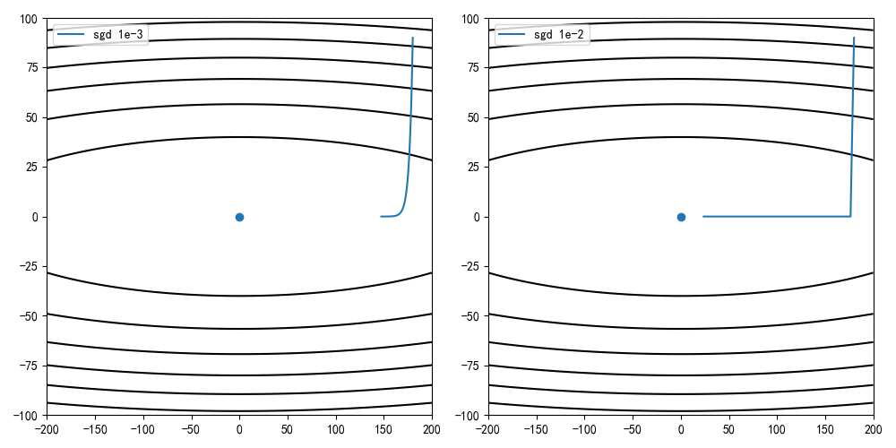
numpy测试 比较标准梯度下降和经典动量更新的损失值收敛梯度,比较不同动量因子(\(\mu\) )的收敛速度
高度计算公式为
\[ h = x^{2} + 50y^{2} \]
实现代码 1 2 3 4 5 6 7 8 9 10 11 12 13 14 15 16 17 18 19 20 21 22 23 24 25 26 27 28 29 30 31 32 33 34 35 36 37 38 39 40 41 42 43 44 45 46 47 48 49 """ 动量测试 """ import matplotlib.pyplot as pltimport numpy as npdef height (x, y ): return x ** 2 + 50 * y ** 2 def gradient (x ): return np.array([2 * x[0 ], 100 * x[1 ]]) def sgd (x_start, lr, epochs=100 ): dots = [x_start] x = x_start.copy() for i in range (epochs): grad = gradient(x) x -= grad * lr dots.append(x.copy()) if abs (np.sum (grad)) < 1e-6 : break return np.array(dots) def sgd_momentum (x_start, lr, epochs=100 , mu=0.5 ): dots = [x_start] x = x_start.copy() v = 0 for i in range (epochs): grad = gradient(x) v = v * mu - lr * grad x += v dots.append(x.copy()) if abs (np.sum (grad)) < 1e-6 : break return np.array(dots)
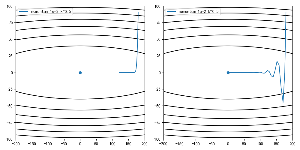
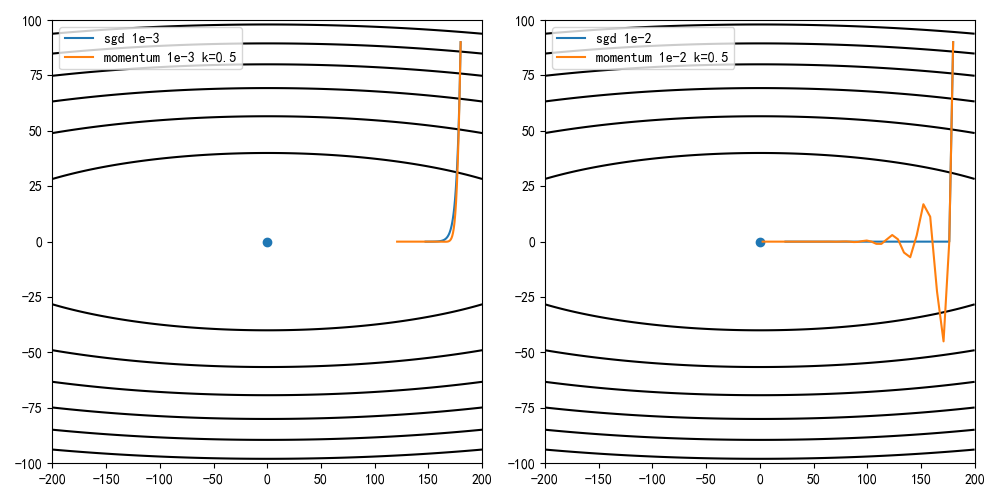
sgd vs momentum 设定学习率为0.001/0.01,动量因子为0.5,迭代100次的收敛情况
由结果可知,相同学习率和迭代数的情况下动量更新能够比标准梯度下降达到更快的收敛速度
1 2 3 4 5 6 7 8 9 10 11 12 13 14 15 16 17 18 19 20 21 22 23 24 25 26 27 28 29 30 31 32 33 34 35 36 37 38 39 40 41 42 43 44 45 46 47 48 49 50 51 52 53 def draw(X, Y, Z, *arr): sgd_dot_list , sgd_label_list, momentum_dot_list, momentum_label_list = arr fig = plt.figure(figsize=(10 , 5 )) plt .subplot(121 ) item = sgd_dot_list[0 ] label = sgd_label_list[0 ] plt .plot(item[:, 0 ], item[:, 1 ], label=label) item = momentum_dot_list[0 ] label = momentum_label_list[0 ] plt .plot(item[:, 0 ], item[:, 1 ], label=label) plt .contour(X, Y, Z, colors='black') plt .scatter(0 , 0 ) plt .legend() plt .subplot(122 ) item = sgd_dot_list[1 ] label = sgd_label_list[1 ] plt .plot(item[:, 0 ], item[:, 1 ], label=label) item = momentum_dot_list[1 ] label = momentum_label_list[1 ] plt .plot(item[:, 0 ], item[:, 1 ], label=label) plt .contour(X, Y, Z, colors='black') plt .scatter(0 , 0 ) plt .legend() plt .show() if __name__ == '__main__': x = np.linspace(-200 , 200 , 1000 ) y = np.linspace(-100 , 100 , 1000 ) X , Y = np.meshgrid(x, y) Z = height(X, Y) x_start = np.array([180 , 90 ], dtype=np.float) epochs = 100 mu = 0 .5 lr_list = [1e-3, 1e-2] sgd_label_list = ['sgd 1e-3', 'sgd 1e-2'] momentum_label_list = ['momentum 1e-3 k=0.5', 'momentum 1e-2 k=0.5'] sgd_dot_list = [] momentum_dot_list = [] for item in lr_list: sgd_dot_list .append(sgd(x_start, item, epochs=epochs)) momentum_dot_list .append(sgd_momentum(x_start, item, epochs=epochs, mu=mu)) draw (X, Y, Z, sgd_dot_list, sgd_label_list, momentum_dot_list, momentum_label_list)
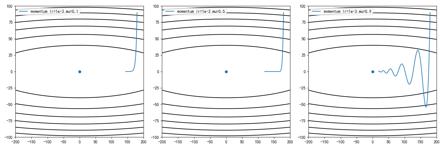
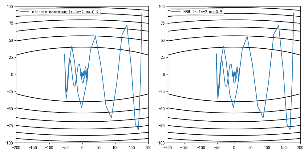
不同动量因子 设定学习率为0.001,动量因子为0.1/0.5,0.9,计算迭代100次后的收敛情况
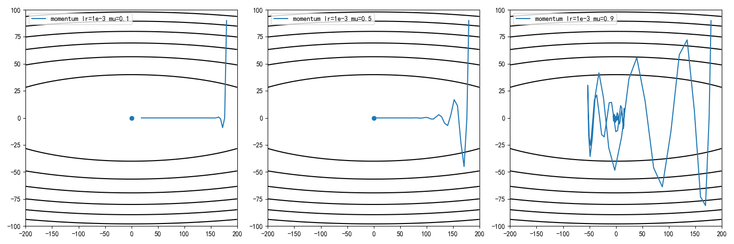
设定学习率为0.01,动量因子为0.1/0.5,0.9,计算迭代100次后的收敛情况
从训练结果可知,动量因子增大能够加快收敛速度,但同时收敛曲线更加动荡
1
2
3
4
5
6
7
8
9
10
11
12
13
14
15
16
17
18
19
20
21
22
23
24
25
26
27
28
29
30
31
32
33
34
35
36
37
38
39
40
41
42
43
44
45
46
47
48
49
50
def draw(X, Y, Z, *arr): momentum_dot_list , momentum_label_list = arr fig = plt.figure(figsize=(15 , 5 )) plt .subplot(131 ) item = momentum_dot_list[0 ] label = momentum_label_list[0 ] plt .plot(item[:, 0 ], item[:, 1 ], label=label) plt .contour(X, Y, Z, colors='black') plt .scatter(0 , 0 ) plt .legend() plt .subplot(132 ) item = momentum_dot_list[1 ] label = momentum_label_list[1 ] plt .plot(item[:, 0 ], item[:, 1 ], label=label) plt .contour(X, Y, Z, colors='black') plt .scatter(0 , 0 ) plt .legend() plt .subplot(133 ) item = momentum_dot_list[2 ] label = momentum_label_list[2 ] plt .plot(item[:, 0 ], item[:, 1 ], label=label) plt .contour(X, Y, Z, colors='black') plt .scatter(0 , 0 ) plt .legend() plt .show() if __name__ == '__main__': x = np.linspace(-200 , 200 , 1000 ) y = np.linspace(-100 , 100 , 1000 ) X , Y = np.meshgrid(x, y) Z = height(X, Y) x_start = np.array([180 , 90 ], dtype=np.float) epochs = 100 mu_list = [0.1, 0.5, 0.9] momentum_label_list = ['momentum lr=1e-3 mu=0.1', 'momentum lr=1e-3 mu=0.5', 'momentum lr=1e-3 mu=0.9'] momentum_dot_list = [] for item in mu_list: momentum_dot_list .append(sgd_momentum(x_start, 1 e-2 , epochs=epochs, mu=item)) draw (X, Y, Z, momentum_dot_list, momentum_label_list)
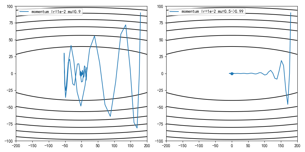
优化方法 动量因子增大能够带来更快的收敛速度,同时也带来了更动荡的收敛曲线
造成收敛曲线不稳定的原因在于累计速度和当前更新方向不一致,这是因为早期小批量图片计算的梯度不能够正确拟合全部图片导致的
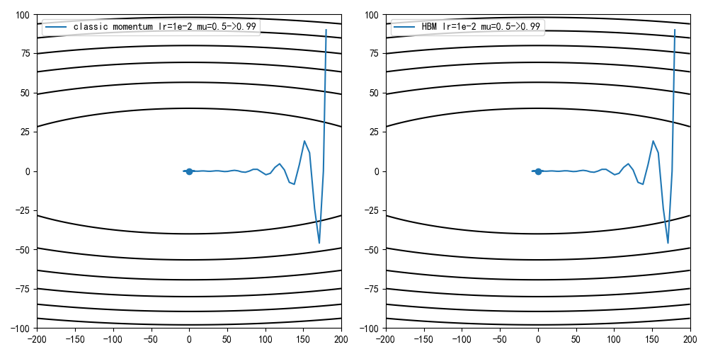
参考学习率退火 ,在早期设置一个较小的动量因子,随着迭代次数增加慢慢增大。比如设置mu=0.5,每轮迭代增加0.01,当mu=0,99时不再增加
1
2
3
4
5
6
7
8
9
10
11
12
13
14
15
16
def sgd_momentum_v2 (x_start, lr, epochs=100 ): dots = [x_start] x = x_start.copy() v = 0 mu = 0 .5 for i in range(epochs): grad = gradient(x) v = v * mu - lr * grad x += v dots .append(x.copy()) if abs(np.sum(grad)) < 1 e-6 : break if mu < 0 .99 : mu += 0 .01 return np.array(dots)
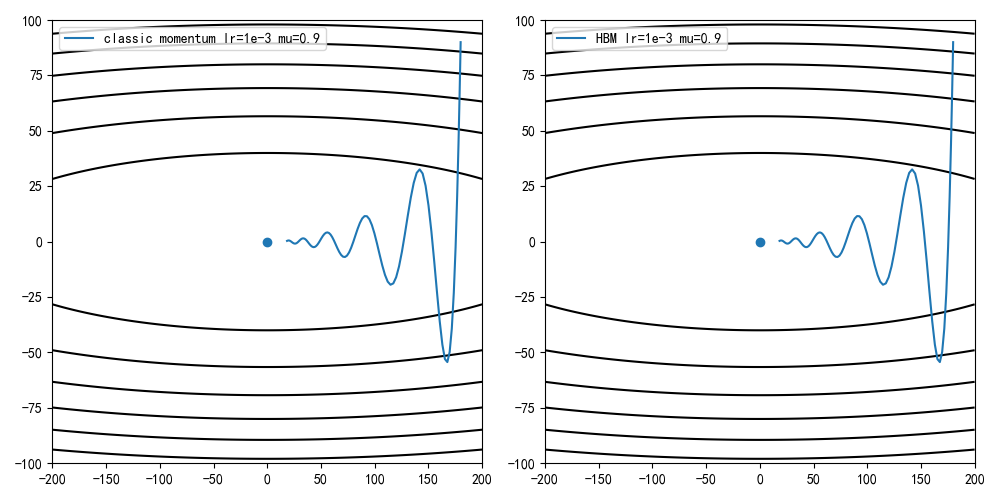
pytorch实现 torch.optim.SGD 实现的动量更新公式有别于经典动量,使用的是重球法(heavy ball method,简称HBM)
\[ v_{t} = \mu v_{t-1} + \triangledown f(w_{t-1})\\ w_{t} = w_{t-1} - lr v_{t} \]
其效果和经典动量类似
1
2
3
4
5
6
7
8
9
10
11
12
13
14
15
def sgd_momentum_v3(x_start, lr, epochs=100 , mu=0.5 ): dots = [x_start] x = x_start.copy () v = 0 for i in range (epochs): grad = gradient(x) v = v * mu + grad x -= lr * v dots.append (x.copy ()) if abs (np .sum (grad)) < 1e-6 : break <!-- if mu < 0.99 : mu += 0.01 --> return np .array (dots)
小结 动量更新方法能够有效的加速训练过程,但需要注意学习率和动量因子的配合
相关阅读