Densely Connected Convolutional Networks
原文地址:Densely Connected Convolutional Networks
摘要
Recent work has shown that convolutional networks can be substantially deeper, more accurate, and efficient to train if they contain shorter connections between layers close to the input and those close to the output. In this paper, we embrace this observation and introduce the Dense Convolutional Network (DenseNet), which connects each layer to every other layer in a feed-forward fashion. Whereas traditional convolutional networks with \(L\) layers have \(L\) connections—one between each layer and its subsequent layer—our network has \(\frac {L(L+1)}{2}\) direct connections. For each layer, the feature-maps of all preceding layers are used as inputs, and its own feature-maps are used as inputs into all subsequent layers. DenseNets have several compelling advantages: they alleviate the vanishing-gradient problem, strengthen feature propagation, encourage feature reuse, and substantially reduce the number of parameters. We evaluate our proposed architecture on four highly competitive object recognition benchmark tasks (CIFAR-10, CIFAR-100, SVHN, and ImageNet). DenseNets obtain significant improvements over the state-of-the-art on most of them, whilst requiring less computation to achieve high performance. Code and pre-trained models are available at https://github.com/liuzhuang13/DenseNet.
最近的研究表明,如果卷积网络在靠近输入端的层和靠近输出端的层之间包含短连接,那么卷积网络可以更深、更准确、更有效地进行训练。在本文中,我们接受了这一观察,并介绍了密集卷积网络(DenseNet),它以前馈方式将每层连接到后续每一层。传统的卷积网络有\(L\)层,共\(L\)个连接,而我们的网络有\(\frac {L(L+1)}{2}\)个连接。对于每层而言,之前所有层的输出特征图都作为输入,其输出的特征图作为所有后续层的输入。DenseNet有几个引人注目的优点:它们减轻了梯度消失的问题,加强了特征传播,鼓励特征重用,并大大减少了参数数量。我们在四个极具竞争力的目标识别基准任务(CIFAR-10、CIFAR-100、SVHN和ImageNet)上评估我们提出的架构。DenseNets在大多数方面都获得了显著的改进,并且仅需要更少的计算来实现高性能。代码和预训练模型已开源:https://github.com/liuzhuang13/DenseNet
DenseNet
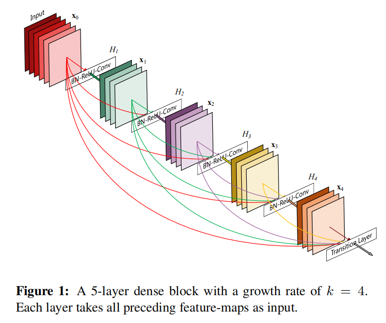
DenseNet(Dense Convolutional Network)通过连接(concatenating)不同层输出的方式,将之前所有层的输出都作为当前层的输入。对于第\(l\)层而言,其包含了\(l\)个输入,由之前所有卷积块输出的特征图组成;而它输出的特征图作为后续\(L-l\)个层的输入数据,所以一个\(L\)层DenseNet共有\(\frac {L(L+1)}{2}\)个连接
ResNet vs. DenseNet
假定输入图像\(x_{0}\),网络包含\(L\)层,每层实现了一个非线性转换\(H_{l}(\cdot )\),其中\(l\)表示层下标,\(H\)是一个复合函数,第\(l\)层的输出称为\(x_{l}\)
对于ResNet而言,其输出等于
\[ x_{l} = H_{l}(x_{l-1}) + x_{l-1} \]
对于DenseNet而言,其输出等于
\[ x_{l} = H_{l}([x_{0}, x_{1}, ..., x_{l-1}]) \]
其中\([x_{0}, x_{1}, ..., x_{l-1}]\)表示前面\(0, ..., (l-1)\)层输出特征图的连接
复合函数
\(H_{l}(\cdot)\)由3个连续执行的操作组成:
- 批量处理(
BN) - 激活函数(
ReLU) - 卷积操作(\(3\times 3\)
Conv)
dense block/transition layer
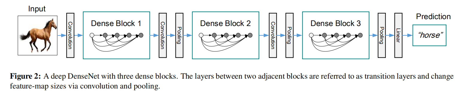
DenseNet由多个dense block和transition layer组成。在dense block中执行密集连接操作,在transition layer中执行特征图减半操作。其中transition层由以下操作组成:
- 批量处理(
BN) - \(1\times 1\)卷积操作
- \(2\times 2\)平均池化操作
Growth rate
假定每个函数\(H_{l}\)生成\(k\)个特征图,那么第\(l\)层得到\(k_{0}+k\times (l-1)\)个特征图,其中\(k_{0}\)表示输入层的深度,超参数\(k\)称为网络学习率(growth rate of the network)
bottleneck layer
论文将\(1\times 1\)卷积层作用于\(3\times 3\)卷积层之前,固定输出\(4k\)个特征图,以此来控制\(3\times 3\)卷积层的输入特征图深度。所以将\(1\times 1\)卷积层称之为瓶颈层(bottleneck layer),其\(H_{l}\)实现为BN-ReLU-Conv(1x1)-BN-ReLU-Conv(3x3),称这个版本模型为DenseNet-B
Compression
除了在Bottleneck Block中控制\(3\times 3\)卷积层的输入特征图数量外,还通过transition layer来减少特征图数目。假定一个dense block输出\(m\)个特征图,经过transition layer计算后得到\(\left \lfloor \theta m \right \rfloor\),其中\(0<\theta \leq 1\)。称\(\theta<1\)的模型为DenseNet-C,论文使用\(\theta = 0.5\)进行实验,称该模型为DenseNet-BC
实现细节
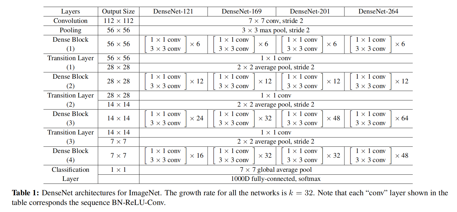
论文提出了两个版本的DenseNet:3个Dense Block或者4个Dense Block。其4个Dense Block的实现细节如下:
- 输入大小为\(224\times 224\)
- 第一个卷积层使用\(2k\)个滤波器,大小为\(7\times 7\),步长为\(2\)
数据集
分别使用了CIFAR-10/100、SVHN以及ImageNet进行测试
CIFAR
- \(32\times 32\)大小彩色图像
CIFAR-10(C10)包含10类,CIFAR-100(C100)包含100类5万张训练图像,1万张测试图像
SVHN
街景门牌号码数据集(The Street View House Numbers DataSet)
- \(32\times 32\)大小彩色图像
73257张训练集、26032张测试集以及531131张图片用于额外训练
ImageNet
ILSVRC 2012分类数据集
120万张训练图片5万张验证图片- 共
1000类
训练
训练参数
对于CIFAR和SVHN数据集
- 批量大小:
64 - 训练次数:
300(CIFAR)和40(SVHN) - 初始学习率
0.1,迭代50%以及75%次后除以10
对于ImageNet
- 批量大小:
256 - 训练次数:
90 - 初始学习率
0.1,迭代30以及60次后除以10
其他训练参数如下:
- 权重衰减:
1e-4 Nesterov动量:0.9
训练结果
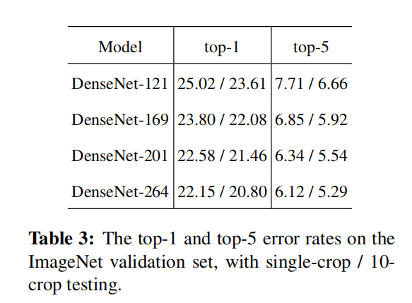
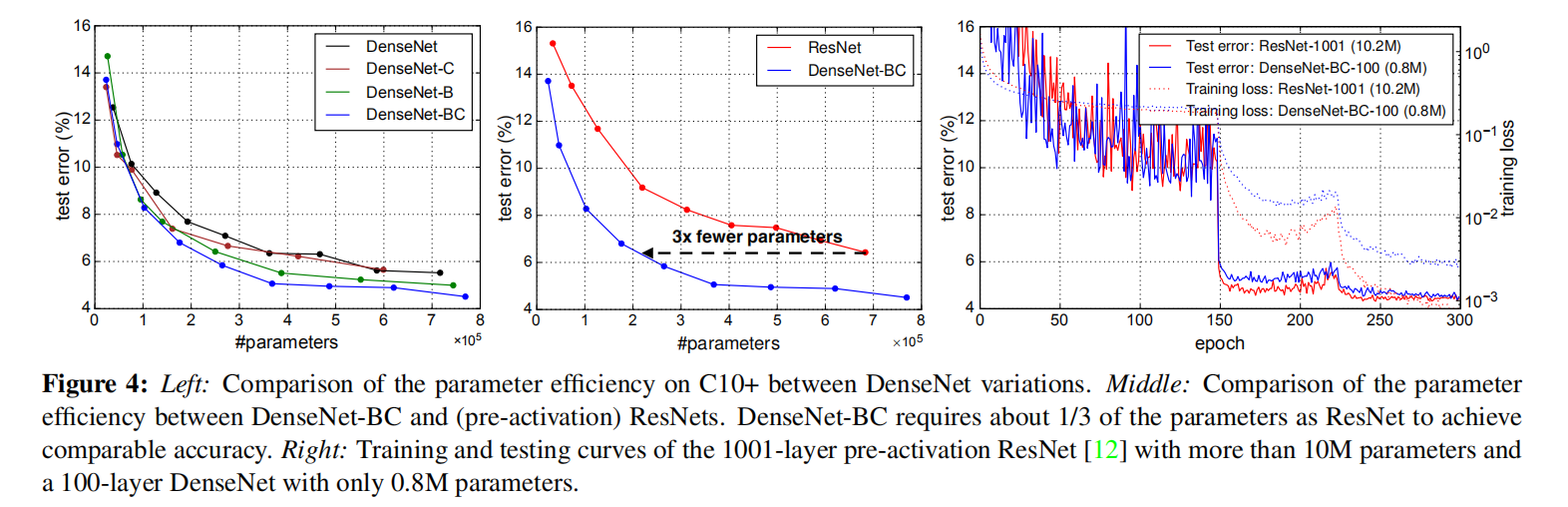
比较不同深度的DenseNet模型Top-1和Top-5误差率,如下表所示
比较各个模型基于不同参数数目/flops以及top-1误差率的结果,如下表所示
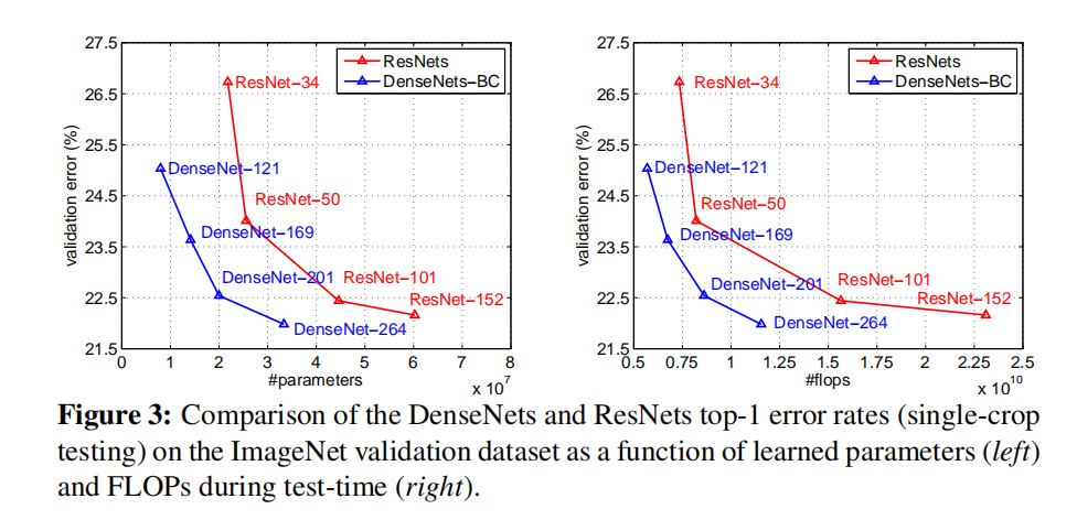
DenseNet通过Dense Block和Transition Layer,相比于ResNet,使用更少的参数数目就能够实现相似的检测精度。实验结果如下表所示
小结
自定义了DenseNet实现,参考zjZSTU/ResNet
各模型大小及Flops如下:
1 | densenet_121: 5.731 GFlops - 30.437 MB |