1
2
3
4
5
6
7
8
9
10
11
12
13
14
15
16
17
18
19
20
21
22
23
24
25
26
27
28
29
30
31
32
33
34
35
36
37
38
39
40
41
42
43
44
45
46
47
48
49
50
51
52
53
54
55
56
57
58
59
60
61
62
63
64
65
66
67
68
69
70
71
72
73
74
75
76
77
78
79
80
81
82
83
84
85
86
87
88
89
90
91
92
93
94
95
96
97
98
99
100
101
102
103
104
105
106
107
108
109
110
111
112
113
114
115
116
117
|
from lr_classifier import LogisticClassifier
import numpy as np
import math
import matplotlib.pyplot as plt
import warnings
warnings.filterwarnings("ignore")
def two_cate_linear():
    x1 = np.linspace(20, 40, num=200)[np.random.choice(200, 120)]
    y1 = np.linspace(20, 40, num=200)[np.random.choice(200, 120)]

    x2 = np.linspace(-10, 10, num=200)[np.random.choice(200, 120)]
    y2 = np.linspace(-10, 10, num=200)[np.random.choice(200, 120)]

    x = np.vstack((np.concatenate((x1, x2)), np.concatenate((y1, y2)))).T
    y = np.concatenate((np.zeros(120), np.ones(120)))

    np.random.seed(120)
    np.random.shuffle(x)
    np.random.seed(120)
    np.random.shuffle(y)

    return x[:200], x[200:], y[:200], y[200:]
def cross_validation(x_train, y_train, x_val, y_val, lr_choices, reg_choices, classifier=LogisticClassifier):
results = {}
best_val = -1
best_svm = None
for lr in lr_choices:
for reg in reg_choices:
svm = classifier()
svm.train(x_train, y_train, learning_rate=lr, reg=reg, num_iters=2000, batch_size=30, verbose=True)
y_train_pred = svm.predict(x_train)
y_val_pred = svm.predict(x_val)
train_acc = np.mean(y_train_pred == y_train)
val_acc = np.mean(y_val_pred == y_val)
results[(lr, reg)] = (train_acc, val_acc)
if best_val < val_acc:
best_val = val_acc
best_svm = svm
return results, best_svm, best_val
def compute_accuracy(y, y_pred):
num = y.shape[0]
num_correct = np.sum(y_pred == y)
acc = float(num_correct) / num
return acc
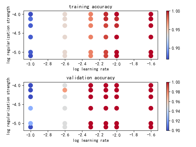
def plot(results):
x_scatter = [math.log10(x[0]) for x in results]
y_scatter = [math.log10(x[1]) for x in results]
marker_size = 100
colors = [results[x][0] for x in results]
plt.subplot(2, 1, 1)
plt.scatter(x_scatter, y_scatter, marker_size, c=colors, cmap=plt.cm.coolwarm)
plt.colorbar()
plt.xlabel('log learning rate')
plt.ylabel('log regularization strength')
plt.title('training accuracy')
colors = [results[x][1] for x in results]
plt.subplot(2, 1, 2)
plt.scatter(x_scatter, y_scatter, marker_size, c=colors, cmap=plt.cm.coolwarm)
plt.colorbar()
plt.xlabel('log learning rate')
plt.ylabel('log regularization strength')
plt.title('validation accuracy')
plt.show()
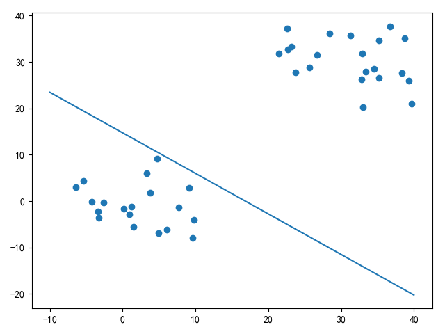
def plot_v2(x, w, b):
plt.scatter(x[:, 0], x[:, 1])
x = np.linspace(-10, 40, num=200)
y = (-x * w[0] - b) / w[1]
plt.plot(x, y)
plt.show()
if __name__ == '__main__':
x_train, x_test, y_train, y_test = two_cate_linear()
lr_choices = [1e-3, 2.5e-3, 5e-3, 7.5e-3, 1e-2, 2.5e-2]
reg_choices = [8e-6, 1e-5, 2.5e-5, 5e-5, 7.5e-5, 1e-4]
results, best_classifier, best_val = cross_validation(x_train, y_train, x_test, y_test, lr_choices, reg_choices)
plot(results)
plot_v2(x_test, best_classifier.W, best_classifier.b)
for k in results.keys():
lr, reg = k
train_acc, val_acc = results[k]
print('lr = %f, reg = %f, train_acc = %f, val_acc = %f' % (lr, reg, train_acc, val_acc))
print('最好的设置是: lr = %f, reg = %f' % (best_classifier.lr, best_classifier.reg))
print('最好的测试精度: %f' % best_val)
|