[译]Identity Mappings in Deep Residual Networks
原文地址:Identity Mappings in Deep Residual Networks
Abstract
摘要
Deep residual networks [1] have emerged as a family of extremely deep architectures showing compelling accuracy and nice convergence behaviors. In this paper, we analyze the propagation formulations behind the residual building blocks, which suggest that the forward and backward signals can be directly propagated from one block to any other block, when using identity mappings as the skip connections and after-addition activation. A series of ablation experiments support the importance of these identity mappings. This motivates us to propose a new residual unit, which makes training easier and improves generalization. We report improved results using a 1001-layer ResNet on CIFAR-10 (4.62% error) and CIFAR-100, and a 200-layer ResNet on ImageNet. Code is available at: https://github.com/KaimingHe/resnet-1k-layers.
深度残差网络[1]已经成为一个极深架构家族,显示出令人信服的准确性和良好的收敛性。本文分析了残差构建块的传播公式,认为当使用恒等式映射作为跳跃连接时,在加法激活后,前向和后向信号可以从一个块直接传播到任何其他块。一系列消融实验证明了恒等式映射的重要性。这促使我们提出一种新的残差单元,使训练更容易,并提高了泛化能力。我们在CIFAR-10 (4.62%的误差)和CIFAR-100上使用1001层ResNet,在ImageNet上使用200层ResNet,报告了改进的结果。代码地址:https://github.com/KaimingHe/resnet-1k-layers
Introduction
引言
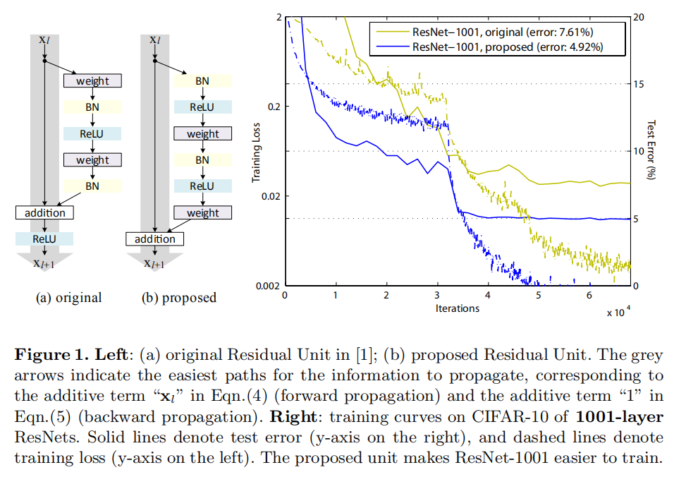
Deep residual networks (ResNets) [1] consist of many stacked “Residual Units”. Each unit (Fig. 1 (a)) can be expressed in a general form:
深度残差网络(ResNets)[1]包含了许多堆叠的“残差单元”。每个单元(图1(a))可以用以下公式表达:
\[ y_{l} = h(x_{l}) + F(x_{l}, W_{l}) \\ x_{l+1} = f(y_{l}) \]
where \(x_{l}\) and \(x_{l+1}\) are input and output of the \(l\)-th unit, and \(F\) is a residual function. In [1], \(h(x_{l}) = x_{l}\) is an identity mapping and \(f\) is a ReLU [2] function.
其中\(x_{l}\)和\(x_{l+1}\)是第\(l\)个单元的输入和输出,\(F\)是一个残差函数。在[1]中,\(h(x_{l})=x_{l}\),表示恒等式映射,\(f\)是ReLU函数
ResNets that are over 100-layer deep have shown state-of-the-art accuracy for several challenging recognition tasks on ImageNet [3] and MS COCO [4] competitions. The central idea of ResNets is to learn the additive residual function \(F\) with respect to \(h(x_{l})\), with a key choice of using an identity mapping \(h(x_{l}) = x_{l}\) .This is realized by attaching an identity skip connection (“shortcut”).
超过100层的ResNets在ImageNet[3]和MS COCO[4]的几个挑战赛上实现了最好的结果。其核心思想是学习关于\(h(x_{l})\)和使用恒等式映射\(h(x_{l})=x_{l}\)的加法残差函数\(F\)。这些通过恒等式映射跳跃连接(快捷连接)实现
In this paper, we analyze deep residual networks by focusing on creating a “direct” path for propagating information — not only within a residual unit, but through the entire network. Our derivations reveal that if both \(h(x_{l})\) and \(f(y_{l})\) are identity mappings, the signal could be directly propagated from one unit to any other units, in both forward and backward passes. Our experiments empirically show that training in general becomes easier when the architecture is closer to the above two conditions.
在本文中,我们通过创建一条“直接”路径来分析深层残差网络,该路径不仅在残差单元内传播信息,而且在整个网络中传播信息。我们的推导表明,如果\(h(x_{l})\)和\(f(y_{l})\)都是恒等式映射,信号可以从一个单元直接传播到任何其他单元,无论是向前还是向后。我们的实验表明,当架构更接近上述两个条件时,训练通常会变得更容易
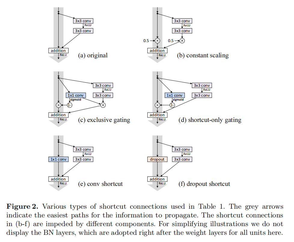
To understand the role of skip connections, we analyze and compare various types of \(h(x_{l})\). We find that the identity mapping \(h(x_{l}) = x_{l}\) chosen in [1] achieves the fastest error reduction and lowest training loss among all variants we investigated, whereas skip connections of scaling, gating [5,6,7], and 1×1 convolutions all lead to higher training loss and error. These experiments suggest that keeping a “clean” information path (indicated by the grey arrows in Fig. 1, 2, and 4) is helpful for easing optimization.
为了理解跳跃连接的作用,我们分析并比较了各种类型的\(h(x_{l})\)。我们发现在[1]中选择的恒等式映射\(h(x_{l}) = x_{l}\)在我们研究的所有变量中实现了最快的误差减少和最低的训练损失,而缩放、门控[5,6,7]和1×1卷积等跳跃连接都导致更高的训练损失和误差。这些实验表明,保持“干净”的信息路径(由图1、2和4中的灰色箭头表示)有助于加快优化过程
To construct an identity mapping \(f(y_{l}) = y_{l}\) , we view the activation functions (ReLU and BN [8]) as “pre-activation” of the weight layers, in contrast to conventional wisdom of “post-activation”. This point of view leads to a new residual unit design, shown in (Fig. 1(b)). Based on this unit, we present competitive results on CIFAR-10/100 with a 1001-layer ResNet, which is much easier to train and generalizes better than the original ResNet in [1]. We further report improved results on ImageNet using a 200-layer ResNet, for which the counterpart of [1] starts to overfit. These results suggest that there is much room to exploit the dimension of network depth, a key to the success of modern deep learning.
为了构建一个恒等式映射\(f(y_{l}) = y_{l}\),我们将激活函数(ReLU和BN [8])视为权重层的“预激活”,这与“后激活”的传统观点相反。这一观点导致了新的残差单元设计,如图1(b)所示。基于这一单元,我们在CIFAR-10/100上展示了具有1001层ResNet的竞争结果,这比[1]中的原始ResNet更易于训练和推广。我们进一步报告了在使用200层ResNet在ImageNet上的改进结果,[1]设计的网络开始过拟合。这些结果表明,网络深度维度有很大的开发空间,这是现代深度学习成功的关键
Analysis of Deep Residual Networks
深度残差网络的分析
The ResNets developed in [1] are modularized architectures that stack building blocks of the same connecting shape. In this paper we call these blocks “Residual Units”. The original Residual Unit in [1] performs the following computation:
在[1]实现的ResNets是模块化的体系结构,它堆叠了相同连接形状的构建块。在本文中,我们称这些块为“残差单元”。[1]中的原始残差单元执行以下计算:
\[ y_{l} = h(x_{l}) + F(x_{l}, W_{l})\ \ \ \ \ \ (1) \\ x_{l+1} = f(y_{l})\ \ \ \ \ (2) \]
Here \(x_{l}\) is the input feature to the \(l\)-th Residual Unit. \(W_{l} = {W_{l},k|_{1≤k≤K}}\) is a set of weights (and biases) associated with the \(l\)-th Residual Unit, and \(K\) is the number of layers in a Residual Unit (\(K\) is 2 or 3 in [1]). \(F\) denotes the residual function, e.g., a stack of two \(3×3\) convolutional layers in [1]. The function \(f\) is the operation after element-wise addition, and in [1] \(f\) is ReLU. The function \(h\) is set as an identity mapping: \(h(x_{l}) = x_{l}\).\(^{1}\)
\(x_{l}\)表示第\(l\)个残差单元的输入特征。\(W_{l} = {W_{l},k|_{1≤k≤K}}\)是第\(l\)个残差单元的一组权重(以及偏差),\(K\)是残差单元的层数(在1中\(K=2/3\))。\(F\)表示残差函数,比如,在[1]中堆叠两个\(3\times 3\)卷积层。函数\(f\)是元素相加后的操作,在[1]中\(f\)是ReLU。函数\(h\)被设置为标识映射:\(h(x_{l}) = x_{l}\)。\(^{1}\)
If \(f\) is also an identity mapping: \(x_{l}+1 ≡ y_{l}\), we can put Eqn.(2) into Eqn.(1) and obtain:
如果\(f\)也是一个恒等式映射: \(x_{l}+1 ≡ y_{l}\),那么结合等式(2)和等式(1)可得:
\[ x_{l+1} = x_{l} + F(x_{l} + W_{l}) \ \ \ \ \ (3) \]
Recursively \((x_{l+2} = x_{l+1} + F(x_{l+1}, W_{l+1}) = x_{l} + F(x_{l} , W_{l}) + F(x_{l+1}, W_{l+1}\) , etc.) we will have:
迭代可得:
\[ x_{L} = x_{l} + \sum_{i=l}^{L-1}F(x_{i}, W_{i}) \ \ \ \ \ (4) \]
for any deeper unit \(L\) and any shallower unit \(l\). Eqn.(4) exhibits some nice properties. (i) The feature \(x_{L}\) of any deeper unit \(L\) can be represented as the feature \(x_{l}\) of any shallower unit \(l\) plus a residual function in a form of \(\sum_{i=l}^{L-1}F\), indicating that the model is in a residual fashion between any units \(L\) and \(l\). (ii) The feature \(x_{L}=x_{0}+\sum_{i=0}^{L-1}F(x_{i}, W_{i})\), of any deep unit \(L\), is the summation of the outputs of all preceding residual functions (plus \(x_{0}\)). This is in contrast to a “plain network” where a feature \(x_{L}\) is a series of matrix-vector products, say, \(\prod _{i=0}^{L-1}W_{i}x_{0}\) (ignoring BN and ReLU)
对于任何更深的单元\(L\)还是更浅的单元\(l\)。等式(4)展示了一些很好的特性。(i) 任何较深单元\(L\)的特征\(x_{L}\)可以表示为任何较浅单元\(l\)的特征\(x_{l}\)加上\(\sum_{i=l}^{L-1}F\)形式的残差函数,表明该模型在任何单元\(L\)和\(l\)中都处于残差形式。(ii) 任何单元\(L\)的特征\(x_{l}=x_{0}+\sum_{i=0}^{l-1}f(x_{i},W_{i})\),是所有前面的残差函数(加上\(x_{0}\))的输出的总和。这与“普通网络”形成对比,在“普通网络”中,其\(x_{L}\)是一系列矩阵向量乘积,比如说,\(\prod _{i=0}^{L-1}W_{i}x_{0}\)(忽略BN和ReLU)
Eqn.(4) also leads to nice backward propagation properties. Denoting the loss function as \(\epsilon\), from the chain rule of backpropagation [9] we have:
等式(4)也具有良好的反向传播特性。根据反向传播[9]的链式法则,将损失函数表示为\(ε\),我们有:
\[ \frac {\partial \epsilon} {\partial x_{l}} = \frac {\partial \epsilon} {\partial x_{L}} \frac {\partial x_{L}}{\partial x_{l}} = \frac {\partial \epsilon} {\partial x_{L}}(1 + \frac {\partial}{x_{l}} \sum_{i=l}^{L-1}F(x_{i}, W_{i})) \ \ \ \ \ (5) \]
Eqn.(5) indicates that the gradient \(\frac {\partial \epsilon}{x_{l}}\) can be decomposed into two additive terms: a term of \(\frac {\partial \epsilon}{x_{L}}\) that propagates information directly without concerning any weight layers, and another term of \(\frac {\partial \epsilon} {\partial x_{L}}( \frac {\partial}{x_{l}} \sum_{i=l}^{L-1}F)\) that propagates through the weight layers. The additive term of \(\frac {\partial \epsilon}{x_{L}}\) ensures that information is directly propagated back to any shallower unit \(l\). Eqn.(5) also suggests that it is unlikely for the gradient \(\frac {\partial \epsilon}{x_{l}}\) to be canceled out for a mini-batch, because in general the term \(\frac {\partial}{x_{l}} \sum_{i=l}^{L-1}F\) cannot be always -1 for all samples in a mini-batch. This implies that the gradient of a layer does not vanish even when the weights are arbitrarily small.
等式(5)表明梯度\(\frac {\partial \epsilon}{x_{l}}\)可以分解成两个加法项:\(\frac {\partial \epsilon}{x_{L}}\)直接传播梯度到输入,不需要经过权重层,另一个 \(\frac {\partial \epsilon} {\partial x_{L}}( \frac {\partial}{x_{l}} \sum_{i=l}^{L-1}F)\)通过权重层传播梯度。\(\frac {\partial \epsilon}{x_{L}}\) 确保了信息直接传播回任何较浅的单位\(l\)。等式(5)还表明,对于小批量样本而言,\(\frac {\partial}{x_{l}} \sum_{i=l}^{L-1}F\)不可能总数为-1,所以梯度\(\frac {\partial \epsilon}{x_{l}}\)不太可能为0。这意味着即使权重再小,层的梯度也不会消失
\(^{1}\) It is noteworthy that there are Residual Units for increasing dimensions and reducing feature map sizes [1] in which h is not identity. In this case the following derivations do not hold strictly. But as there are only a very few such units (two on CIFAR and three on ImageNet, depending on image sizes [1]), we expect that they do not have the exponential impact as we present in Sec. 3. One may also think of our derivations as applied to all Residual Units within the same feature map size.
值得注意的是,存在用于增加维度和减小特征图尺寸的残差单位[1],其中\(h\)不是恒等的。在这种情况下,下列推导并不严格成立。但是,由于只有极少数这样的单元(两个在CIFAR上,三个在ImageNet上,具体取决于图像大小[1]),我们预计它们不会像我们在第3节中介绍的那样具有指数级的影响。可以认为我们的推导仅适用于相同特征图大小的残差单位
Discussion
讨论
Eqn.(4) and Eqn.(5) suggest that the signal can be directly propagated from any unit to another, both forward and backward. The foundation of Eqn.(4) is two identity mappings: (i) the identity skip connection \(h(x_{l}) = x_{l}\) , and (ii) the condition that \(f\) is an identity mapping.
等式(4)和(5)证明了信号可以从任何单元直接传播到另一个单元,不论向前和向后操作。等式(4)的基础是两个恒等式映射:(i) 恒等跳跃连接\(h(x_{l}) = x_{l}\),(ii) 函数\(f\)是恒等式映射
These directly propagated information flows are represented by the grey arrows in Fig. 1, 2, and 4. And the above two conditions are true when these grey arrows cover no operations (expect addition) and thus are “clean”. In the following two sections we separately investigate the impacts of the two conditions.
这些直接传播的信息流由图1、2和4中的灰色箭头表示。当这些灰色箭头不包含任何操作(除了加法操作)时,上述两个条件成立,因此是“干净的”。在接下来的两节中,我们将分别研究这两种情况的影响
On the Importance of Identity Skip Connections
恒等式连接的重要性
Let’s consider a simple modification, \(h(x_{l}) = λ_{l}x_{l}\), to break the identity shortcut:
进行一个简单的修改:\(h(x_{l}) = λ_{l}x_{l}\),以打破恒等式连接
\[ x_{l+1} = \lambda_{l}x_{l} + F(x_{L}, W_{l}) \ \ \ \ \ (6) \]
where \(λ_{l}\) is a modulating scalar (for simplicity we still assume \(f\) is identity). Recursively applying this formulation we obtain an equation similar to Eqn. (4): \(x_{L} = (\prod _{i=l}^{L-1}\lambda_{i})x_{l} + \sum_{i=l}^{L-1}(\prod_{j=i+1}^{L-1}\lambda_{j})F(x_{i}, W_{i})\), or simply:
其中\(λ_{l}\)是一个调节标量(为简化起见,仍旧假设\(f\)是恒等式)。递归实现上述公式得到类似于等式(4)的结果:\(x_{L} = (\prod _{i=l}^{L-1}\lambda_{i})x_{l} + \sum_{i=l}^{L-1}(\prod_{j=i+1}^{L-1}\lambda_{j})F(x_{i}, W_{i})\),或者简化为:
\[ x_{L} = (\prod _{i=l}^{L-1}\lambda_{i})x_{l} + \sum_{i=l}^{L-1} \hat{F}(x_{i}, W_{i}) \ \ \ \ \ (7) \]
where the notation \(\hat{F}\) absorbs the scalars into the residual functions. Similar to Eqn.(5), we have backpropagation of the following form:
其中记号\(\hat{F}\)将标量放置进残差函数中。实现的反向传播公式如下:
\[ \frac {\partial \epsilon}{\partial x_{l}} = \frac {\partial \epsilon}{\partial x_{L}}((\prod_{i=l}^{L-1} \lambda_{i}) + \frac {\partial}{\partial x_{l}} \sum_{i=l}^{L-1}\hat{F} (x_{i}, W_{i})) \ \ \ \ \ (8) \]
Unlike Eqn.(5), in Eqn.(8) the first additive term is modulated by a factor \(\prod_{i=l}^{L-1} \lambda_{i}\). For an extremely deep network (\(L\) is large), if \(λ_{i} > 1\) for all \(i\), this factor can be exponentially large; if \(λ_{i} < 1\) for all \(i\), this factor can be exponentially small and vanish, which blocks the backpropagated signal from the shortcut and forces it to flow through the weight layers. This results in optimization difficulties as we show by experiments.
不像等式(5),在等式(8)中,第一个加法项乘以一个因子\(\prod_{i=l}^{L-1} \lambda_{i}\)。对于极深网络\(L\)而言,如果所有的\(\lambda_{i} > 1\),那么这个因子将会指数大;如果所有\(\lambda_{i} < 1\),那么这个因子将会指数小,甚至消失。它会阻止来自快捷方式的反向传播信号,并强制其通过权重层。实验结果表明,这给优化带来了困难
In the above analysis, the original identity skip connection in Eqn.(3) is replaced with a simple scaling \(h(x_{l}) = \lambda_{l} x_{l}\). If the skip connection \(h(x_{l})\) represents more complicated transforms (such as gating and \(1×1\) convolutions), in Eqn.(8) the first term becomes \(\prod_{i=l}^{L-1}{h}'_{i}\) where \({h}'\) is the derivative of \(h\). This product may also impede information propagation and hamper the training procedure as witnessed in the following experiments.
在上面的分析中,原来的恒等式跳跃连接(等式(3))被一个简单的缩放 \(h(x_{l}) = \lambda_{l} x_{l}\)所替代。如果这个跳跃连接\(h(x_{l})\)表示更复杂的转换(比如门控或者\(1\times 1\)卷积),那么等式(8)的第一项变成\(\prod_{i=l}^{L-1}{h}'_{i}\),其中\({h}'\)是\(h\)的导数。实验证明,这种实现也有可能阻止信息传播,妨碍训练过程
Experiments on Skip Connections
跳跃连接实验
We experiment with the 110-layer ResNet as presented in [1] on CIFAR-10 [10]. This extremely deep ResNet-110 has 54 two-layer Residual Units (consisting of 3×3 convolutional layers) and is challenging for optimization. Our implementation details (see appendix) are the same as [1]. Throughout this paper we report the median accuracy of 5 runs for each architecture on CIFAR, reducing the impacts of random variations.
我们在CIFAR-10上对[1]中提出的110层ResNet进行了实验。ResNet-110具有54个两层残差单元(由3×3卷积层组成),对优化具有挑战性。我们的实现细节(见附录)与[1]相同。在本文中,我们报告了CIFAR上每个架构5次运行的中间精度,减少了随机变化的影响
Though our above analysis is driven by identity \(f\), the experiments in this section are all based on \(f\) = ReLU as in [1]; we address identity f in the next section. Our baseline ResNet-110 has 6.61% error on the test set. The comparisons of other variants (Fig. 2 and Table 1) are summarized as follows:
尽管上述分析是由恒等式\(f\)驱动的,但本节中的实验都是基于\(f\)=ReLU,如[1]所示;我们在下一节中讨论恒等式\(f\)。我们的基线ResNet-110在测试集上有6.61%的误差。其他变体(图2和表1)的比较总结如下:
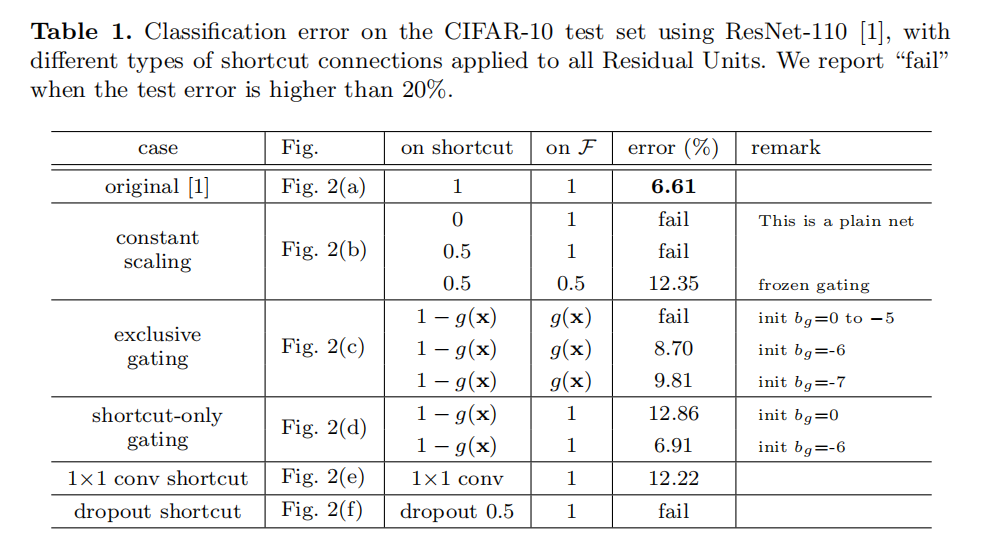
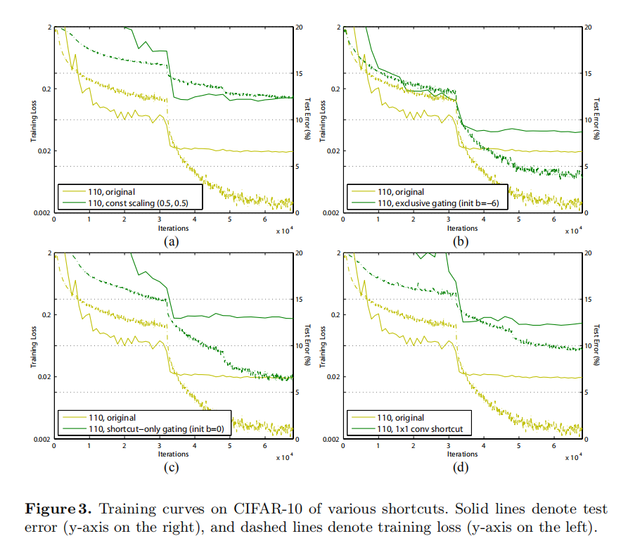
Constant scaling. We set \(λ = 0.5\) for all shortcuts (Fig. 2(b)). We further study two cases of scaling \(F\): (i) \(F\) is not scaled; or (ii) \(F\) is scaled by a constant scalar of \(1−λ = 0.5\), which is similar to the highway gating [6,7] but with frozen gates. The former case does not converge well; the latter is able to converge, but the test error (Table 1, 12.35%) is substantially higher than the original ResNet-110. Fig 3(a) shows that the training error is higher than that of the original ResNet-110, suggesting that the optimization has difficulties when the shortcut signal is scaled down.
常量缩放。我们设置所有快捷连接的\(λ=0.5\)(图2(b))。我们进一步研究了两种缩放\(F\)的情况:(i)\(F\)没有缩放;或(ii)\(F\)使用\(1-λ=0.5\)的常量因子,这与highway gating[6,7]相似,但门是冻结的。前一种情况收敛不好;后一种情况能够收敛,但测试误差(表1,12.35%)大大高于原始ResNet-110。图3(a)显示训练误差高于原始ResNet-110,这表明当缩小快捷连接信号时,优化有困难
Exclusive gating. Following the Highway Networks [6,7] that adopt a gating mechanism [5], we consider a gating function \(g(x) = \sigma (W_{g}x + b_{g})\) where a transform is represented by weights \(W_{g}\) and biases \(b_{g}\) followed by the sigmoid function \(\sigma(x) = \frac {1}{1+e^{-x}}\). In a convolutional network g(x) is realized by a 1×1 convolutional layer. The gating function modulates the signal by element-wise multiplication.
专有门控。参考Highway Networks [6,7]的门控机制[5],考虑一个门控函数 \(g(x) = \sigma (W_{g}x + b_{g})\),对于权重\(W_{g}\)和偏置值\(b_{g}\)实现sigmoid函数\(\sigma(x) = \frac {1}{1+e^{-x}}\)。在卷积网络中,\(g(x)\)由1×1卷积层实现。门控函数通过逐元素乘法来控制信号
We investigate the “exclusive” gates as used in [6,7] — the \(F\) path is scaled by \(g(x)\) and the shortcut path is scaled by \(1−g(x)\). See Fig 2(c). We find that the initialization of the biases \(b_{g}\) is critical for training gated models, and following the guidelines$^{2} $ in [6,7], we conduct hyper-parameter search on the initial value of bg in the range of 0 to -10 with a decrement step of -1 on the training set by crossvalidation. The best value (−6 here) is then used for training on the training set, leading to a test result of 8.70% (Table 1), which still lags far behind the ResNet-110 baseline. Fig 3(b) shows the training curves. Table 1 also reports the results of using other initialized values, noting that the exclusive gating network does not converge to a good solution when \(b_{g}\) is not appropriately initialized.
\(F\)路径被缩放为\(g(x)\),快捷连接路径被缩放为\(1-g(x)\),见图2(c)。我们发现偏置值\(b_{g}\)的初始化对于训练门控模型是至关重要的,并且遵循[6,7]中的准则\(^{2}\),我们对0到-10范围内的\(b_{g}\)初始值进行超参数搜索,并对交叉验证后的训练集进行-1的递减。然后将最佳值(此处为-6)用于训练集上的训练,得到8.70%的测试结果(表1),这仍然远远落后于ResNet-110基线。图3(b)显示了训练曲线。表1还报告了使用其他初始化值的结果,注意到当\(b_{g}\)未正确初始化时,专有门控网络不会收敛到一个好的解决方案
The impact of the exclusive gating mechanism is two-fold. When \(1 − g(x)\) approaches 1, the gated shortcut connections are closer to identity which helps information propagation; but in this case \(g(x)\) approaches 0 and suppresses the function \(F\). To isolate the effects of the gating functions on the shortcut path alone, we investigate a non-exclusive gating mechanism in the next.
排他性浇口机制的影响是双重的。当\(1-g(x)\)接近1时,门控快捷连接更接近于有助于信息传播的标识;但在这种情况下,\(g(x)\)接近0并抑制函数\(F\)。为了分离选通函数单独对快捷路径的影响,我们在下一步研究了一种非排他选通机制。
专有门控机制的影响是双重的。当\(1-g(x)\)接近1时,门控快捷连接更接近于帮助信息传播的恒等式;但在这种情况下,\(g(x)\)接近0,抑制了函数\(F\)。为了分离门控函数单独对快捷连接路径的影响,我们在下一步研究了一种非专门门控机制
Shortcut-only gating. In this case the function \(F\) is not scaled; only the shortcut path is gated by \(1−g(x)\). See Fig 2(d). The initialized value of \(b_{g}\) is still essential in this case. When the initialized \(b_{g}\) is 0 (so initially the expectation of \(1 − g(x)\) is 0.5), the network converges to a poor result of 12.86% (Table 1). This is also caused by higher training error (Fig 3(c)).
仅快捷连接连通。在这种情况下,函数\(F\)没有被缩放;只有快捷路径被\(1-g(x)\)连通。见图2(d)。在这种情况下,\(b_{g}\)的初始化值仍然是必需的。当初始化\(b_{g}\)为0时(因此最初\(1-g(x)\)的期望值为0.5),网络收敛到12.86%(表1)。这也是由较高的训练误差引起的(图3(c))
When the initialized \(b_{g}\) is very negatively biased (e.g., −6), the value of \(1−g(x)\) is closer to 1 and the shortcut connection is nearly an identity mapping. Therefore, the result (6.91%, Table 1) is much closer to the ResNet-110 baseline.
当初始化的\(b_{g}\)为负偏置时(例如-6),值\(1-g(x)\)更接近1,快捷方式连接几乎是一个恒等式映射。因此,结果(6.91%,表1)更接近ResNet-110基线
1×1 convolutional shortcut. Next we experiment with 1×1 convolutional shortcut connections that replace the identity. This option has been investigated in [1] (known as option C) on a 34-layer ResNet (16 Residual Units) and shows good results, suggesting that 1×1 shortcut connections could be useful. But we find that this is not the case when there are many Residual Units. The 110-layer ResNet has a poorer result (12.22%, Table 1) when using 1×1 convolutional shortcuts. Again, the training error becomes higher (Fig 3(d)). When stacking so many Residual Units (54 for ResNet-110), even the shortest path may still impede signal propagation. We witnessed similar phenomena on ImageNet with ResNet-101 when using 1×1 convolutional shortcuts.
1×1卷积快捷连接。接下来,我们用1×1卷积快捷连接来代替恒等式。该选项已在1中的34层ResNet (16个残差单元)上进行了研究,并显示出良好的结果,表明1×1快捷连接可能是有用的。但我们发现,当有许多残差单位时,情况并非如此。当使用1×1卷积快捷方式时,110层ResNet的结果较差(12.22%,表1)。同样,训练误差变得更高(图3(d))。当堆叠如此多的残差单元(ResNet-110为54)时,即使是最短的路径也可能阻碍信号传播。当使用1×1卷积快捷键时,我们在带有ResNet-101的ImageNet上看到了类似的现象
Dropout shortcut. Last we experiment with dropout [11] (at a ratio of 0.5) which we adopt on the output of the identity shortcut (Fig. 2(f)). The network fails to converge to a good solution. Dropout statistically imposes a scale of λ with an expectation of 0.5 on the shortcut, and similar to constant scaling by 0.5, it impedes signal propagation.
随机失活快捷连接。最后,我们用11中的随机失活进行实验,我们在恒等式快捷连接的输出上采用了这一方法(图2(f))。网络未能收敛到一个好的解决方案。从统计角度来看,随机失活会在快捷连接上施加一个\(\lambda = 0.5\)的缩放因子,与0.5的常数缩放相似,它会阻碍信号传播
Discussion
讨论
As indicated by the grey arrows in Fig. 2, the shortcut connections are the most direct paths for the information to propagate. Multiplicative manipulations (scaling, gating, 1×1 convolutions, and dropout) on the shortcuts can hamper information propagation and lead to optimization problems.
如图2中的灰色箭头所示,快捷连接是信息传播的最直接路径。对快捷连接的乘法操作(缩放、选通、1×1卷积和随机失活)会阻碍信息传播并导致优化问题
It is noteworthy that the gating and 1×1 convolutional shortcuts introduce more parameters, and should have stronger representational abilities than identity shortcuts. In fact, the shortcut-only gating and 1×1 convolution cover the solution space of identity shortcuts (i.e., they could be optimized as identity shortcuts). However, their training error is higher than that of identity shortcuts, indicating that the degradation of these models is caused by optimization issues, instead of representational abilities.
值得注意的是,门控和1×1卷积快捷连接引入了更多的参数,并且应该比恒等式快捷连接具有更强的表示能力。事实上,仅快捷连接门控和1×1卷积覆盖了恒等式快捷方式的解决方案空间(即它们可以被优化恒等式快捷连接)。然而,它们的训练误差高于恒等式,这表明这些模型的退化是由优化问题引起的,而不是由表征能力引起的
On the Usage of Activation Functions
激活函数的使用
Experiments in the above section support the analysis in Eqn.(5) and Eqn.(8), both being derived under the assumption that the after-addition activation \(f\) is the identity mapping. But in the above experiments \(f\) is ReLU as designed in [1], so Eqn.(5) and (8) are approximate in the above experiments. Next we investigate the impact of \(f\).
上一节的实验证明了公式(5)和(8)中的分析。两者都是在添加后激活\(f\)是恒等式映射的假设下导出的。在上面的实验中,按照[1]中\(f\)是ReLU,所以(5)和(8)在上述实验中是近似的。接下来,我们将研究\(f\)的影响
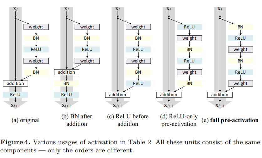
We want to make \(f\) an identity mapping, which is done by re-arranging the activation functions (ReLU and/or BN). The original Residual Unit in [1] has a shape in Fig. 4(a) — BN is used after each weight layer, and ReLU is adopted after BN except that the last ReLU in a Residual Unit is after elementwise addition (\(f\) = ReLU). Fig. 4(b-e) show the alternatives we investigated, explained as following.
我们希望通过重新排列激活函数(ReLU和/或BN)来实现恒等式映射。[1]中的原始残差单元具有图4(a)中的形状——在每个权重层之后使用BN,并且在BN之后采用ReLU,除了残差单元中的最后一个ReLU是在元素相加之后(\(f\) = ReLU)。图4(b-e)显示了我们研究的替代方案,解释如下
Experiments on Activation
激活实验
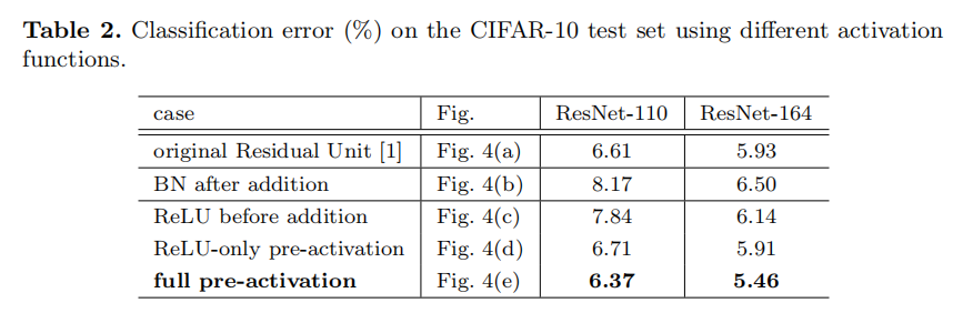
In this section we experiment with ResNet-110 and a 164-layer Bottleneck [1] architecture (denoted as ResNet-164). A bottleneck Residual Unit consist of a 1×1 layer for reducing dimension, a 3×3 layer, and a 1×1 layer for restoring dimension. As designed in [1], its computational complexity is similar to the two-3×3 Residual Unit. More details are in the appendix. The baseline ResNet-164 has a competitive result of 5.93% on CIFAR-10 (Table 2).
本节中我们用ResNet-110和164层Bottleneck[1]体系结构(表示为ResNet-164)进行实验。一个Bottleneck残差单元由1×1(降维)、3×3和1×1(恢复维度)组成。如[1]中所设计的,其计算复杂性类似于2个3×3组成的残差单元。更多细节见附录。基线ResNet-164在CIFAR-10上的训练结果为5.93%(表2)
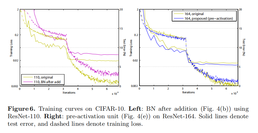
BN after addition. Before turning \(f\) into an identity mapping, we go the opposite way by adopting BN after addition (Fig. 4(b)). In this case \(f\) involves BN and ReLU. The results become considerably worse than the baseline (Table 2). Unlike the original design, now the BN layer alters the signal that passes through the shortcut and impedes information propagation, as reflected by the difficulties on reducing training loss at the beginning of training (Fib. 6 left).
相加后执行BN。在把\(f\)转换成一个恒等式映射之前,我们实现相反的操作,在加法之后采用BN(图4(b))。在这种情况下,\(f\)涉及BN和ReLU。结果变得比基线差得多(表2)。与最初的设计不同,现在的BN层改变了通过捷径的信号,阻碍了信息的传播,正如在训练开始时减少训练损失的困难所反映的(Fib。6左)
ReLU before addition. A naive choice of making \(f\) into an identity mapping is to move the ReLU before addition (Fig. 4(c)). However, this leads to a non-negative output from the transform \(F\), while intuitively a “residual” function should take values in (−∞, +∞). As a result, the forward propagated signal is monotonically increasing. This may impact the representational ability, and the result is worse (7.84%, Table 2) than the baseline. We expect to have a residual function taking values in (−∞, +∞). This condition is satisfied by other Residual Units including the following ones.
加法前执行ReLU。将\(f\)转换成恒等式映射的一个简单选择是在加法操作之前实现ReLU(图4(c))。然而,这导致变换\(F\)的非负输出,而直观上“残差”函数应该取值为(∞,+∞)。结果,正向传播信号单调增加。这可能会影响代表性能力,结果比基线更差(7.84%,表2)。我们希望有一个取值为(−∞, +∞)的残差函数
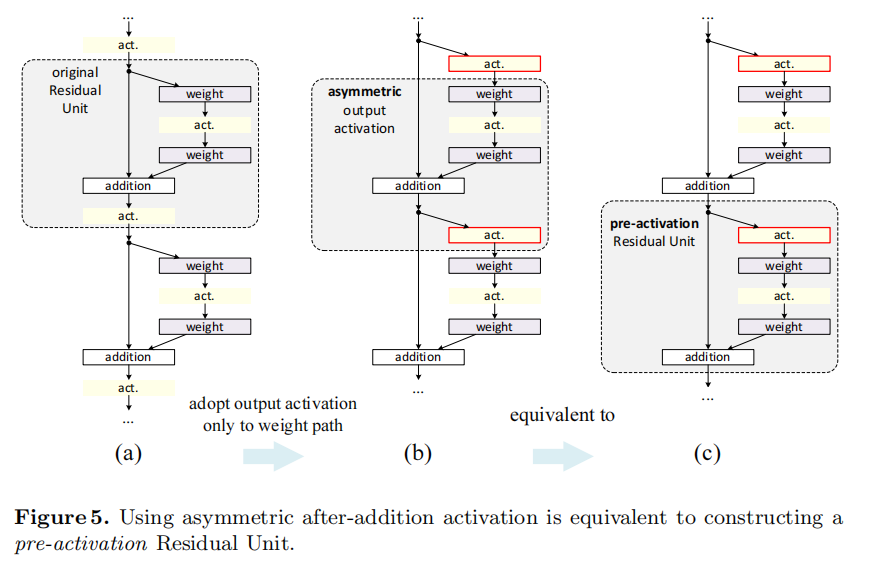
Post-activation or pre-activation? In the original design (Eqn.(1) and Eqn.(2)), the activation \(x_{l+1} = f(y_{l})\) affects both paths in the next Residual Unit: \(y_{l+1} = f(y_{l}) + F(f(y_{l}), W_{l+1})\). Next we develop an asymmetric form where an activation \(\hat{f}\) only affects the \(F\) path: \(y_{l+1} = y_{l} + F(\hat{f}(y_{l}), W_{l+1})\), for any \(l\) (Fig. 5 (a) to (b)). By renaming the notations, we have the following form:
前激活还是后激活? 对于原始设计(等式(1)和等式(5)),激活\(x_{l+1} = f(y_{l})\)会影响下一个残差单位中的两条路径: \(y_{l+1} = f(y_{l}) + F(f(y_{l}), W_{l+1})\)。接下来,我们开发了一种非对称形式,其中激活只影响\(F\)路径: \(y_{l+1} = y_{l} + F(\hat{f}(y_{l}), W_{l+1})\)。对于任何$ l $(图5 (a)至(b))。通过重命名符号,我们得到了以下形式:
\[ x_{l+1} = x_{l} + F(\hat{f}(x_{l}), W_{l}) \ \ \ \ \ (9) \]
It is easy to see that Eqn.(9) is similar to Eqn.(4), and can enable a backward formulation similar to Eqn.(5). For this new Residual Unit as in Eqn.(9), the new after-addition activation becomes an identity mapping. This design means that if a new after-addition activation \(\hat{f}\) is asymmetrically adopted, it is equivalent to recasting \(\hat{f}\) as the pre-activation of the next Residual Unit. This is illustrated in Fig. 5.
很容易看出等式(9)类似于等式(4),并且能够实现类似于等式(5)的反向公式。对于这个新的残差单元,如等式(9)所示。新的激活后相加成为恒等式映射。这种设计意味着,如果非对称地采用新的激活后相加$ \(的话,它相当于将\) $重铸为下一个残差单元的预激活。如图5中所示
The distinction between post-activation/pre-activation is caused by the presence of the element-wise addition. For a plain network that has N layers, there are N − 1 activations (BN/ReLU), and it does not matter whether we think of them as post- or pre-activations. But for branched layers merged by addition, the position of activation matters.
激活后/激活前的区别是由元素相加的存在引起的。对于一个有N层的普通网络,有\(N-1\)个激活(BN/ReLU),我们认为它们是后激活还是前激活并不重要。但是对于通过添加合并的分支层,激活的位置很重要
We experiment with two such designs: (i) ReLU-only pre-activation (Fig. 4(d)), and (ii) full pre-activation (Fig. 4(e)) where BN and ReLU are both adopted before weight layers. Table 2 shows that the ReLU-only pre-activation performs very similar to the baseline on ResNet-110/164. This ReLU layer is not used in conjunction with a BN layer, and may not enjoy the benefits of BN [8].
我们用两种设计进行实验:(i)仅ReLU预激活(图4(d)),和(ii)完全预激活(图4(e)),其中BN和ReLU都在加权层之前被采用。表2显示,仅ReLU预激活的性能与ResNet-110/164上的基线非常相似。此ReLU层不与BN层结合使用,可能无法享受BN [8]的优势
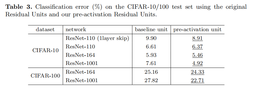
Somehow surprisingly, when BN and ReLU are both used as pre-activation, the results are improved by healthy margins (Table 2 and Table 3). In Table 3 we report results using various architectures: (i) ResNet-110, (ii) ResNet-164, (iii) a 110-layer ResNet architecture in which each shortcut skips only 1 layer (i.e., a Residual Unit has only 1 layer), denoted as “ResNet-110(1layer)”, and (iv) a 1001-layer bottleneck architecture that has 333 Residual Units (111 on each feature map size), denoted as “ResNet-1001”. We also experiment on CIFAR-100. Table 3 shows that our “pre-activation” models are consistently better than the baseline counterparts. We analyze these results in the following.
不知何故,令人惊讶的是,当BN和ReLU都被用作预激活时,结果得到改善(表2和表3)。在表3中,我们使用各种结构进行实验:(i) ResNet-110,(ii) ResNet-164,(iii)110层ResNet,其中每个快捷连接仅跳过1层(即,残差单元只有1层),表示为“ResNet-110(1层)”,以及(iv)1001层bottleneck结构,具有333个残差单元(每个特征图大小有111个),表示为“ResNet-1001”。我们还在CIFAR-100上进行了实验。表3显示,我们的“预激活”模型始终优于基线模型。我们在下面分析这些结果
Analysis
分析
We find the impact of pre-activation is twofold. First, the optimization is further eased (comparing with the baseline ResNet) because f is an identity mapping. Second, using BN as pre-activation improves regularization of the models.
我们发现预激活的影响是双重的。首先,优化被进一步简化(与基线ResNet相比),因为\(f\)是一个恒等式映射。第二,使用BN作为预激活改善了模型的正则化
Ease of optimization. This effect is particularly obvious when training the 1001-layer ResNet. Fig. 1 shows the curves. Using the original design in [1], the training error is reduced very slowly at the beginning of training. For \(f\) = ReLU, the signal is impacted if it is negative, and when there are many Residual Units, this effect becomes prominent and Eqn.(3) (so Eqn.(5)) is not a good approximation. On the other hand, when \(f\) is an identity mapping, the signal can be propagated directly between any two units. Our 1001-layer network reduces the training loss very quickly (Fig. 1). It also achieves the lowest loss among all models we investigated, suggesting the success of optimization.
易于优化。当训练1001层的ResNet时,这种效果尤其明显。图1显示了曲线。使用[1]中的原始设计,训练误差在训练开始时非常缓慢地减小。对于\(f\) = ReLU,如果\(f\)为负的话信号受到影响,当有许多残差单位时,这种影响变得尤为显著,等式(3) (以及等式(5))都不是一个好的近似值。另一方面,当\(f\)是恒等式映射时,信号可以在任意两个单元之间直接传播。我们的1001层网络非常快速地减少了训练损失(图1)。在我们研究的所有模型中,它还实现了最低的损失,这表明优化是成功的
We also find that the impact of \(f\) = ReLU is not severe when the ResNet has fewer layers (e.g., 164 in Fig. 6(right)). The training curve seems to suffer a little bit at the beginning of training, but goes into a healthy status soon. By monitoring the responses we observe that this is because after some training, the weights are adjusted into a status such that \(y_{l}\) in Eqn.(1) is more frequently above zero and \(f\) does not truncate it (\(x_{l}\) is always non-negative due to the previous ReLU, so \(y_{l}\) is below zero only when the magnitude of \(F\) is very negative). The truncation, however, is more frequent when there are 1000 layers.
我们还发现,当ResNet具有较少的层(例如,图6中的164(右))时,\(f\)=ReLU的影响并不严重。训练曲线在训练开始时似乎会受到一点影响,但很快就会进入健康状态。通过监测反应,我们观察到这是因为在一些训练之后,权重被调整到这样一种状态,即方程1中的\(y_{l}\)更经常地高于零,并且\(F\)不截断它(由于先前的ReLU,\(x_{l}\)总是非负的,所以只有当\(F\)的幅度非常负时,\(y_{l}\)才低于零)。然而,当有1000层时,截断更加频繁
Reducing overfitting. Another impact of using the proposed pre-activation unit is on regularization, as shown in Fig. 6 (right). The pre-activation version reaches slightly higher training loss at convergence, but produces lower test error. This phenomenon is observed on ResNet-110, ResNet-110(1-layer), and ResNet-164 on both CIFAR-10 and 100. This is presumably caused by BN’s regularization effect [8]. In the original Residual Unit (Fig. 4(a)), although the BN normalizes the signal, this is soon added to the shortcut and thus the merged signal is not normalized. This unnormalized signal is then used as the input of the next weight layer. On the contrary, in our pre-activation version, the inputs to all weight layers have been normalized.
减少过拟合。使用预激活单元的另一个影响是正则化,如图6(右)所示。预激活版本在收敛时达到稍高的训练损失,但产生较低的测试误差。这种现象在ResNet-110、ResNet-110(1层)和ResNet-164上都可以在CIFAR-10和100上观察到。这大概是由BN的正則化效应造成的[8]。在原始残差单元(图4(a))中,尽管BN对信号进行了归一化,但是这很快被添加到快捷连接中,因此合并的信号没有被归一化。这个未标准化的信号然后被用作下一个权重层的输入。相反,在我们的预激活版本中,所有权重层的输入都已标准化
Results
结果
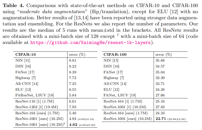
Comparisons on CIFAR-10/100. Table 4 compares the state-of-the-art methods on CIFAR-10/100, where we achieve competitive results. We note that we do not specially tailor the network width or filter sizes, nor use regularization techniques (such as dropout) which are very effective for these small datasets. We obtain these results via a simple but essential concept — going deeper. These results demonstrate the potential of pushing the limits of depth.
CIFAR-10/100的比较。表4比较了CIFAR-10/100上的最新方法,在这些方法中,我们获得了有竞争力的结果。我们注意到,我们没有专门定制网络宽度或滤波器大小,也没有使用正则化技术(如随机失活),这些技术对这些小数据集非常有效。我们通过一个简单但重要的概念获得这些结果 - 更深。这些结果显示了突破深度极限的潜力
Comparisons on ImageNet. Next we report experimental results on the 1000- class ImageNet dataset [3]. We have done preliminary experiments using the skip connections studied in Fig. 2 & 3 on ImageNet with ResNet-101 [1], and observed similar optimization difficulties. The training error of these non-identity shortcut networks is obviously higher than the original ResNet at the first learning rate (similar to Fig. 3), and we decided to halt training due to limited resources. But we did finish a “BN after addition” version (Fig. 4(b)) of ResNet-101 on ImageNet and observed higher training loss and validation error. This model’s single-crop (224×224) validation error is 24.6%/7.5%, vs. the original ResNet-101’s 23.6%/7.1%. This is in line with the results on CIFAR in Fig. 6 (left).
在ImageNet上进行比较。接下来,我们报告在1000类ImageNet数据集[3]上的实验结果。我们已经使用图2和图3中研究的跳跃连接,用ResNet-101 [1]在ImageNet上进行了初步实验,并观察到类似的优化困难。这些非恒等式快捷连接网络的训练误差在第一次学习时明显高于原始ResNet(类似于图3),并且由于资源有限,我们决定停止训练。但我们确实在ImageNet上完成了ResNet-101的“激活后BN”版本(图4(b)),并观察到更高的训练损失和验证错误。该模型的单裁剪(224×224)验证误差为24.6%/7.5%,而原始ResNet-101的误差为23.6%/7.1%。这与图6(左)中的CIFAR结果一致
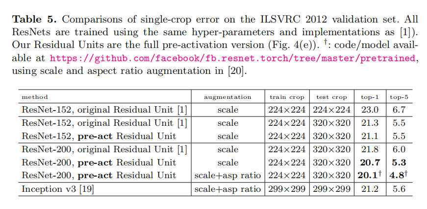
Table 5 shows the results of ResNet-152 [1] and ResNet-2003 , all trained from scratch. We notice that the original ResNet paper [1] trained the models using scale jittering with shorter side s ∈ [256, 480], and so the test of a 224×224 crop on s = 256 (as did in [1]) is negatively biased. Instead, we test a single 320×320 crop from s = 320, for all original and our ResNets. Even though the ResNets are trained on smaller crops, they can be easily tested on larger crops because the ResNets are fully convolutional by design. This size is also close to 299×299 used by Inception v3 [19], allowing a fairer comparison.
表5显示了ResNet-152 [1]和ResNet-2003的结果,都是从零开始训练的。我们注意到,原始的ResNet论文[1]使用短边s ∈ [256,480]的比例抖动来训练模型,因此在s = 256上对224×224裁剪的测试(如在[1中所做的)是负偏差的。相反,我们从s = 320中测试单个320×320裁剪,用于所有原始和我们的ResNets。尽管ResNet是在较小的裁剪上训练的,但是它们可以很容易地在较大的裁剪上测试,因为ResNet是全卷积的。这一尺寸也接近Incetption_v3 [19]所用的299×299,允许更公平的比较
The original ResNet-152 [1] has top-1 error of 21.3% on a 320×320 crop, and our pre-activation counterpart has 21.1%. The gain is not big on ResNet-152 because this model has not shown severe generalization difficulties. However, the original ResNet-200 has an error rate of 21.8%, higher than the baseline ResNet-152. But we find that the original ResNet-200 has lower training error than ResNet-152, suggesting that it suffers from overfitting.
原始的ResNet-152 [1]在320×320裁剪上的top-1误差为21.3%,而预激活的误差为21.1%。ResNet-152的增益不大,因为该模型没有显示出严重的泛化困难。然而,原始ResNet-200的错误率为21.8%,高于基线ResNet-152。但是我们发现原始的ResNet-200比ResNet-152具有更低的训练误差,这表明它遭遇了过拟合
Our pre-activation ResNet-200 has an error rate of 20.7%, which is 1.1% lower than the baseline ResNet-200 and also lower than the two versions of ResNet-152. When using the scale and aspect ratio augmentation of [20,19], our ResNet-200 has a result better than Inception v3 [19] (Table 5). Concurrent with our work, an Inception-ResNet-v2 model [21] achieves a single-crop result of 19.9%/4.9%. We expect our observations and the proposed Residual Unit will help this type and generally other types of ResNets.
我们的预激活ResNet-200的错误率为20.7%,比基线ResNet-200低1.1%,也比ResNet-152的两个版本低。当使用[20,19]的比例和纵横比扩充时,我们的ResNet-200比Inception_v3 [19]有更好的结果(表5)。与我们的工作同时进行的是,Inception-ResNet-v2模型[21]实现了19.9%/4.9%的单一裁剪结果。我们希望我们的观察和建议的残差单元将有助于这种类型和一般其他类型的ResNet
Computational Cost. Our models’ computational complexity is linear on depth (so a 1001-layer net is ∼10× complex of a 100-layer net). On CIFAR, ResNet-1001 takes about 27 hours to train on 2 GPUs; on ImageNet, ResNet-200 takes about 3 weeks to train on 8 GPUs (on par with VGG nets [22]).
计算成本。我们模型的计算复杂度与深度成线性关系(因此1001层网络是100层网络的10倍复杂度)。在CIFAR上,ResNet-1001用2个GPU训练大约需要27个小时;在ImageNet上,ResNet-200需要大约3周时间在8个GPU上进行训练(与VGG[22]一样)
\(^{3}\) The ResNet-200 has 16 more 3-layer bottleneck Residual Units than ResNet-152, which are added on the feature map of 28×28.
\(^{3}\) ResNet-200比ResNet-152多了16个3层bottleneck残差单元,它们被添加在28×28的特征图上
Conclusions
总结
This paper investigates the propagation formulations behind the connection mechanisms of deep residual networks. Our derivations imply that identity shortcut connections and identity after-addition activation are essential for making information propagation smooth. Ablation experiments demonstrate phenomena that are consistent with our derivations. We also present 1000-layer deep networks that can be easily trained and achieve improved accuracy.
本文研究深度残差网络连接机制背后的传播公式。我们的推导表明,恒等式快捷连接和恒等式相加后激活对于使信息传播顺畅至关重要。消融实验证明了与我们的推导一致的现象。我们还提供了1000层的深层网络,可以很容易地进行训练,并提高准确性
Appendix: Implementation Details
附录:实施细节
The implementation details and hyperparameters are the same as those in [1]. On CIFAR we use only the translation and flipping augmentation in [1] for training. The learning rate starts from 0.1, and is divided by 10 at 32k and 48k iterations. Following [1], for all CIFAR experiments we warm up the training by using a smaller learning rate of 0.01 at the beginning 400 iterations and go back to 0.1 after that, although we remark that this is not necessary for our proposed Residual Unit. The mini-batch size is 128 on 2 GPUs (64 each), the weight decay is 0.0001, the momentum is 0.9, and the weights are initialized as in [23].
实施细节和超参数与[1]中的相同。在CIFAR上,我们仅使用[1]中的translation和翻转扩充来进行训练。学习率从0.1开始,在32k和48k迭代中除以10。在[1]之后,对于所有的CIFAR实验,我们在开始的400次迭代中使用较小的学习率0.01来预热训练,然后返回到0.1,尽管我们注意到这对于我们提议的残差单元不是必需的。在2个GPU上进行小批量训练(每个64个),权重衰减为1e-4,动量为0.9,权重初始化如[23]所示
On ImageNet, we train the models using the same data augmentation as in [1]. The learning rate starts from 0.1 (no warming up), and is divided by 10 at 30 and 60 epochs. The mini-batch size is 256 on 8 GPUs (32 each). The weight decay, momentum, and weight initialization are the same as above.
在ImageNet上,我们使用与[1]相同的数据扩充来训练模型。学习率从0.1开始(不预热),在30和60个时期除以10。在8个GPU上进行小批量处理(每个32个)。权重衰减、动量和权重初始化与上面相同
When using the pre-activation Residual Units (Fig. 4(d)(e) and Fig. 5), we pay special attention to the first and the last Residual Units of the entire network. For the first Residual Unit (that follows a stand-alone convolutional layer, conv1), we adopt the first activation right after conv1 and before splitting into two paths; for the last Residual Unit (followed by average pooling and a fully-connected classifier), we adopt an extra activation right after its element-wise addition. These two special cases are the natural outcome when we obtain the pre-activation network via the modification procedure as shown in Fig. 5.
当使用预激活残差单元时(图4(d)(e)和图5),我们特别注意整个网络的第一个和最后一个残差单元。对于第一个残差单元(在独立卷积层conv1之后),我们在conv1之后并在分成两条路径之前采用第一个激活;对于最后一个残差单元(接下来是平均池化和一个全连接分类器),我们在元素相加之后立即采用了一个额外的激活。这两种特殊情况是当我们通过如图5所示的修改过程获得预激活网络时的自然结果
The bottleneck Residual Units (for ResNet-164/1001 on CIFAR) are constructed following [1]. For example, a \(\begin{bmatrix} 3\times 3 & 16\\ 3\times 3 & 16 \end{bmatrix}\) unit in ResNet-110 is replaced with a \(\begin{bmatrix} 1\times 1 & 16\\ 3\times 3 & 16\\ 1\times 1 & 64 \end{bmatrix}\) unit in ResNet-164, both of which have roughly the same number of parameters. For the bottleneck ResNets, when reducing the feature map size we use projection shortcuts [1] for increasing dimensions, and when preactivation is used, these projection shortcuts are also with pre-activation.
作用于CIFAR的ResNet-164/1001使用[1]中的bottleneck残差单元结构.比如,ResNet-110中的\(\begin{bmatrix} 3\times 3 & 16\\ 3\times 3 & 16 \end{bmatrix}\)单元被替换成ResNet-164使用的\(\begin{bmatrix} 1\times 1 & 16\\ 3\times 3 & 16\\ 1\times 1 & 64 \end{bmatrix}\)单元,两者几乎有相同的参数数。对于bottleneck网络,当减少特征图尺寸时,我们使用投影快捷连接方式[1]来增加维度,并且当使用预激活时,这些投影快捷方式也具有预激活