逻辑回归(logistic regression)是分类算法,常用于二元分类
基本求导公式 对数函数求导
\[ y=log_{a}^{x} \Rightarrow {y}'=\frac{1}{xln(a)} \Rightarrow {ln(x)}'=\frac{1}{x} \]
幂函数求导
\[ y=\frac{1}{x^{n}} \Rightarrow {y}'=-\frac{n}{x^{n+1}} \]
指数函数求导
\[ y=n^x \Rightarrow {y}'=n^x \cdot ln(n) \Rightarrow {(e^x)}'=e^x \]
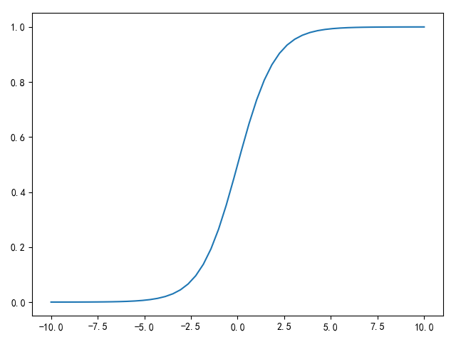
sigmoid函数 sigmoid函数简称为S型函数,也称为logistic函数,公式如下:
\[ g(z)=\frac{1}{1+e^{-z}} \]
\(e^{-z}\) 常写为\(exp(-z)\)
\[ \frac{\varphi }{\varphi z}g(z)=\frac{-1}{(1+e^{-z})^2}\cdot {(e^{-z})}' = \frac{-e^{-z}}{(1+e^{-z})^2}\cdot {(-z)}' = \frac{e^{-z}}{(1+e^{-z})^2} \]
\[ =\frac{1}{1+e^{-z}}\cdot \frac{e^{-z}}{1+e^{-z}} =\frac{1}{1+e^{-z}}\cdot (1-\frac{1}{1+e^{-z}}) =g(z)\cdot (1-g(z)) \]
其实现特性如下:
当输入值大于0时,输出趋近于1 当输入值小于0时,输出趋近于-1 当输入值等于0时,输出为0.5 1 2 3 4 5 6 7 8 9 10 11 12 13 14 15 16 17 18 import matplotlib.pyplot as plt import numpy as np def sigmoid(x): return 1 / (1 + np.exp (-1 * x)) def draw_sigmoid (): x = np.linspace (-10 , 10 ) y = sigmoid (np.array (x)) plt.plot (x, y) plt.show () if __name__ == '__main__' : draw_sigmoid ()
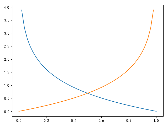
负对数似然代价函数 负对数似然代价函数计算公式如下
\[ cost(h(x;\theta),y)=\left\{\begin{matrix} -ln(h(x;\theta)),y=1 \\ -ln(1-h(x;\theta)),y=0 \end{matrix}\right. \]
分两种情况
判定计算结果是否为1。当计算结果为1时,代价为0,否则代价随\(h(x;\theta)\) 减少而增大 判定计算结果是否为0。当计算结果为0时,代价为0,否则代价随\(h(x;\theta)\) 增大而增大 1 2 3 4 5 6 7 8 9 10 11 12 13 14 15 16 17 18 19 20 import matplotlib.pyplot as pltimport numpy as npdef cost (x): y1 = -1 * np.log(x) y2 = -1 * np.log(1 - x) return y1, y2 def draw_cost(): x = np.linspace(0 , 1 ) y1, y2 = cost (x) plt.plot(x, y1) plt.plot(x, y2) plt.show () if __name__ == '__main__' : draw_cost()
交叉熵损失函数 在二元分类中,结果y取值为0或1,将负对数似然代价函数的两种情况合并在一起得到交叉熵损失函数(cross entropy loss function)
\[ loss(h(x;\theta),y)=-yln(h(x;\theta))-(1-y)ln(1-h(x;\theta)) \]
逻辑回归 逻辑回归的实现就是线性回归加上sigmoid操作,其线性操作如下:
\[ z_{\theta}(x)=\theta^T\cdot x=\theta_{0}\cdot x_{0}+\theta_{1}\cdot x_{1}+...+\theta_{n}\cdot x_{n} \]
逻辑回归模型实现公式如下:
\[ h(x;\theta)=g(z_{\theta}(x))=g(\theta^T\cdot x)=\frac{1}{1+e^{-\theta^T\cdot x}} \]
对逻辑回归模型求导如下:
\[ \frac{\varphi }{\varphi \theta_{i}}h(x;\theta)={h(\theta^T\cdot x)}'={g(\theta^T\cdot x)}' =g(\theta^T\cdot x)\cdot (1-g(\theta^T\cdot x))\cdot {(\theta^T\cdot x)}' \] \[ =g(\theta^T\cdot x)\cdot (1-g(\theta^T\cdot x))\cdot x_{i} =h(x;\theta)\cdot (1-h(x;\theta))\cdot x_{i} \]
逻辑回归利用sigmoid函数进行二元分类,首先对输入数据进行线性运算\(\theta^T\cdot x\) ,再将结果输入sigmoid函数,压缩到\([0,1]\) 范围内,输出结果作为判别概率,表示输出结果为1的可能性,即\(h(x;\theta)=P(y=1|x;\theta)\) ,相对应的输出结果为0的概率为\(P(y=0|x;\theta)=1-h(x;\theta)\)
逻辑回归利用交叉熵损失函数作为二元分类损失函数,公式如下:
\[ J(\theta)=-\frac{1}{N} \sum_{j=1}^{N} \begin{bmatrix} y_{j}ln(h(x_{j};\theta))+(1-y_{j})ln(1-h(x_{j};\theta)) \end{bmatrix} \]
矩阵运算如下:
\[ \Rightarrow J(\theta)= -\frac{1}{N} (Y^T\cdot ln(g(X\cdot \theta))+(1-Y^T)\cdot ln(1-g(X\cdot \theta)) \]
其中\(X\) 大小为\(m\times (n+1)\) ,\(\theta\) 大小为\((n+1)\times 1\) ,\(Y\) 大小为\(m\times 1\) ,\(m\) 表示样本数量,\(n\) 表示权重数量
测试数据 使用numeric类型的德国信用数据,其包含24个变量和一个2类标签 - german.data-numeric
梯度下降 使用批量训练数据进行梯度计算,对损失函数求导如下:
\[ \frac{\varphi }{\varphi \theta_{i}}J(\theta)= -\frac{1}{N} \sum_{j=1}^{N} \begin{bmatrix} y_{j}ln(h(x_{j};\theta))+(1-y_{j})ln(1-h(x_{j};\theta)) \end{bmatrix}' \] \[ =-\frac{1}{N} \sum_{j=1}^{N} \begin{bmatrix} y_{j}\frac{1}{h(x_{j};\theta)}\cdot {h(\theta^T\cdot x)}'+(1-y_{j})\frac{1}{1-h(x_{j};\theta)}\cdot {(1-h(\theta^T\cdot x))}' \end{bmatrix} \] \[ =-\frac{1}{N} \sum_{j=1}^{N} \begin{bmatrix} y_{j}\frac{1}{h(x_{j};\theta)}\cdot h(x_{j};\theta)\cdot (1-h(x_{j};\theta))\cdot x_{j,i}+(1-y_{j})\frac{1}{1-h(x_{j};\theta)}\cdot -h(x_{j};\theta)\cdot (1-h(x_{j};\theta))\cdot x_{j,i} \end{bmatrix} \] \[ =-\frac{1}{N} \sum_{j=1}^{N} \begin{bmatrix} y_{j}\cdot (1-h(x_{j};\theta))\cdot x_{j,i} - (1-y_{j})\cdot h(x_{j};\theta)\cdot x_{j,i} \end{bmatrix} \] \[ =-\frac{1}{N} \sum_{j=1}^{N} \begin{bmatrix} y_{j}\cdot x_{j,i} - h(x_{j};\theta)\cdot x_{j,i} \end{bmatrix} =\frac{1}{N} \sum_{j=1}^{N} \begin{bmatrix} (h(x_{j};\theta)-y_{j})\cdot x_{j,i} \end{bmatrix} \]
其中\(x_{j,i}\) 表示第\(j\) 行第\(i\) 列,矩阵运算如下:
\[ \Rightarrow \frac{\varphi }{\varphi \theta}J(\theta)= \frac{1}{N} X^T\cdot (g(X\cdot \theta)-Y) \]
其中\(X\) 大小为\(m\times (n+1)\) ,\(\theta\) 大小为\((n+1)\times 1\) ,\(Y\) 大小为\(m\times 1\) ,\(m\) 表示样本数量,\(n\) 表示权重数量
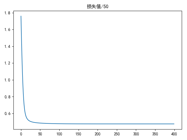
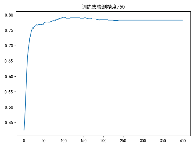
实现 1 2 3 4 5 6 7 8 9 10 11 12 13 14 15 16 17 18 19 20 21 22 23 24 25 26 27 28 29 30 31 32 33 34 35 36 37 38 39 40 41 42 43 44 45 46 47 48 49 50 51 52 53 54 55 56 57 58 59 60 61 62 63 64 65 66 67 68 69 70 71 72 73 74 75 76 77 78 79 80 81 82 83 84 85 86 87 88 89 90 91 92 93 94 95 96 97 98 99 100 101 102 103 104 105 106 107 108 109 110 111 112 113 114 115 116 117 118 119 120 121 122 123 124 125 126 127 128 129 130 131 132 133 134 135 136 137 138 139 140 141 import matplotlib.pyplot as pltimport numpy as npimport pandas as pdfrom sklearn.model_selection import train_test_splitdata_path = '../data/german.data-numeric' def load_data (tsize=0.8 , shuffle=True ): data_list = pd.read_csv(data_path, header=None , sep='\s+' ) data_array = data_list.values height, width = data_array.shape[:2 ] data_x = data_array[:, :(width - 1 )] data_y = data_array[:, (width - 1 )] x_train, x_test, y_train, y_test = train_test_split(data_x, data_y, train_size=tsize, test_size=(1 - tsize), shuffle=shuffle) y_train = np.atleast_2d(np.array(list (map (lambda x: 1 if x == 2 else 0 , y_train)))).T y_test = np.atleast_2d(np.array(list (map (lambda x: 1 if x == 2 else 0 , y_test)))).T return x_train, y_train, x_test, y_test def init_weights (inputs ): """ 初始化权重,符合标准正态分布 """ return np.atleast_2d(np.random.uniform(size=inputs)).T def sigmoid (x ): return 1 / (1 + np.exp(-1 * x)) def logistic_regression (w, x ): """ w大小为(n+1)x1 x大小为mx(n+1) """ z = x.dot(w) return sigmoid(z) def compute_loss (w, x, y ): """ w大小为(n+1)x1 x大小为mx(n+1) y大小为mx1 """ lr_value = logistic_regression(w, x) n = y.shape[0 ] res = -1.0 / n * (y.T.dot(np.log(lr_value)) + (1 - y.T).dot(np.log(1 - lr_value))) return res[0 ][0 ] def compute_gradient (w, x, y ): """ 梯度计算 """ n = y.shape[0 ] lr_value = logistic_regression(w, x) return 1.0 / n * x.T.dot(lr_value - y) def compute_predict_accuracy (predictions, y ): results = predictions > 0.5 res = len (list (filter (lambda x: x[0 ] == x[1 ], np.dstack((results, y))[:, 0 ]))) / len (results) return res def draw (res_list, title=None , xlabel=None , ylabel=None ): if title is not None : plt.title(title) if xlabel is not None : plt.xlabel(xlabel) plt.plot(res_list) plt.show() if __name__ == '__main__' : train_data, train_label, test_data, test_label = load_data() mu = np.mean(train_data, axis=0 ) std = np.std(train_data, axis=0 ) train_data = (train_data - mu) / std test_data = (test_data - mu) / std train_data = np.insert(train_data, 0 , np.ones(train_data.shape[0 ]), axis=1 ) test_data = np.insert(test_data, 0 , np.ones(test_data.shape[0 ]), axis=1 ) lr = 0.01 w = init_weights(train_data.shape[1 ]) epoches = 20000 loss_list = [] accuracy_list = [] loss = 0 best_accuracy = 0 best_w = None for i in range (epoches): loss += compute_loss(w, train_data, train_label) gradient = compute_gradient(w, train_data, train_label) tempW = w - lr * gradient w = tempW if i % 50 == 49 : accuracy = compute_predict_accuracy(logistic_regression(w, train_data), train_label) accuracy_list.append(accuracy) if accuracy > best_accuracy: best_accuracy = accuracy best_w = w.copy() loss_list.append(loss / 50 ) loss = 0 draw(loss_list, title='损失值/50' ) draw(accuracy_list, title='训练集检测精度/50' ) print(max (accuracy_list)) print(compute_predict_accuracy(logistic_regression(best_w, test_data), test_label))
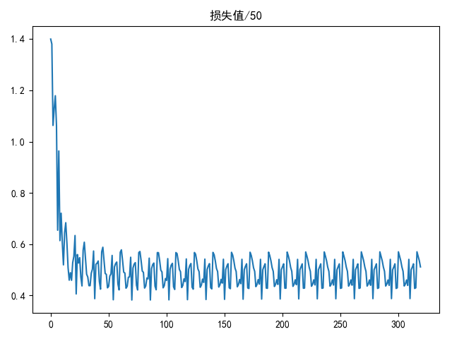
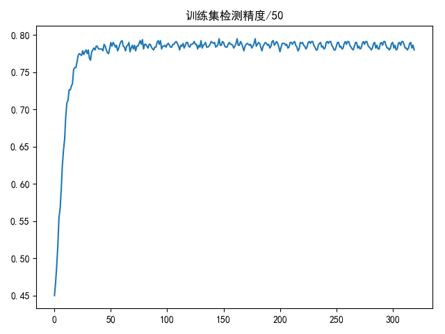
随机梯度下降实现如下
1 2 3 4 5 6 7 8 9 10 11 12 13 14 15 16 17 18 19 20 21 22 23 24 25 26 27 28 29 30 31 32 33 34 35 36 37 38 39 40 41 42 43 44 45 46 47 48 49 50 51 52 53 54 55 56 57 58 59 60 61 62 63 64 65 66 67 68 69 70 71 72 ... import warningswarnings.filterwarnings('ignore' ) ... ... def compute_loss (w, x, y, isBatch=True ): """ w大小为(n+1)x1 x大小为mx(n+1) y大小为mx1 """ lr_value = logistic_regression(w, x) if isBatch: n = y.shape[0 ] res = -1.0 / n * (y.T.dot(np.log(lr_value)) + (1 - y.T).dot(np.log(1 - lr_value))) return res[0 ][0 ] else : res = -1.0 * (y * (np.log(lr_value)) + (1 - y) * (np.log(1 - lr_value))) return res[0 ] def compute_gradient (w, x, y, isBatch=True ): """ 梯度计算 """ lr_value = logistic_regression(w, x) if isBatch: n = y.shape[0 ] return 1.0 / n * x.T.dot(lr_value - y) else : return np.atleast_2d(1.0 * x.T * (lr_value - y)).T ... ... if __name__ == '__main__' : ... ... epoches = 20 num = train_label.shape[0 ] loss_list = [] accuracy_list = [] loss = 0 best_accuracy = 0 best_w = None for i in range (epoches): for j in range (num): loss += compute_loss(w, train_data[j], train_label[j], isBatch=False ) gradient = compute_gradient(w, train_data[j], train_label[j], isBatch=False ) tempW = w - lr * gradient w = tempW if j % 50 == 49 : accuracy = compute_predict_accuracy(logistic_regression(w, train_data), train_label) accuracy_list.append(accuracy) if accuracy > best_accuracy: best_accuracy = accuracy best_w = w.copy() loss_list.append(loss / 50 ) loss = 0 draw(loss_list, title='损失值/50' ) draw(accuracy_list, title='训练集检测精度/50' ) print(max (accuracy_list)) print(compute_predict_accuracy(logistic_regression(best_w, test_data), test_label))
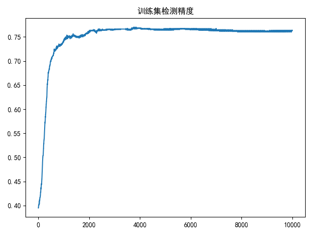
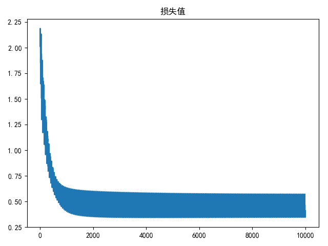
小批量梯度下降结果如下:
1 2 3 4 5 6 7 8 9 10 11 12 13 14 15 16 17 18 19 20 21 22 23 24 25 26 27 28 29 30 31 32 # 计算目标函数/损失函数以及梯度更新 epoches = 200 batch_size = 128 num = train_label.shape[0 ] loss_list = [] accuracy_list = [] loss = 0 best_accuracy = 0 best_w = None for i in range(epoches): for j in range(0 , num, 16 ): loss_list.append(compute_loss(w , train_data [j :j + batch_size ], train_label [j :j + batch_size ], isBatch =True) ) # 计算梯度 gradient = compute_gradient(w , train_data [j :j + batch_size ], train_label [j :j + batch_size ], isBatch =True) # 权重更新 tempW = w - lr * gradient w = tempW # 每个小批次记录一次 # 计算精度 accuracy = compute_predict_accuracy(logistic_regression (w , train_data ) , train_label) accuracy_list.append(accuracy) if accuracy > best_accuracy: best_accuracy = accuracy best_w = w.copy() draw(loss_list, title='损失值') draw(accuracy_list, title='训练集检测精度') print(max(accuracy_list)) print(compute_predict_accuracy(logistic_regression (best_w , test_data ) , test_label))
RuntimeWarning: divide by zero encountered in log 计算损失过程中可能会出现精度错误:
1 data_loss = -1.0 / num_train * np .sum (y_batch * np .log (scores) + (1 - y_batch) * np .log (1 - scores))
修改如下:
1
2
3
4
eplison = 1e-5 scores = self.logistic_regression(X_batch) data_loss = -1.0 / num_train * np .sum (y_batch * np .log (np .maximum(scores, eplison)) + (1 - y_batch) * np .log (np .maximum(1 - scores, eplison)))
小结 逻辑回归二元分类需要注意:
标签值的转换(将两类标签转换成0/1数值) 预测值的计算(计算单个预测值就能判断类别) 相关阅读