直方图

发表于 2019-11-08 更新于 2021-11-21 分类于视觉/vision 阅读次数：

本文字数： 11k 阅读时长 ≈ 20 分钟

以下主要涉及颜色直方图的概念和计算

最开始学习数字图像处理的时候就接触到了直方图的概念，也记录过OpenCV 1.x/2.x的直方图实现代码

颜色/纹理等特征通过直方图的形式能够有效的作用于图像检测/识别算法，所以打算再整理一下相关的概念和实现。参考：

Histogram Equalization
Histogram Calculation
Histogram Comparison
头文件地址：/path/to/opencv-4.0.1/modules/imgproc/include/opencv2/imgproc.hpp
源文件地址：/path/to/opencv-4.0.1/modules/imgproc/src/histogram.cpp

内容列表

什么是直方图？
直方图计算
直方图均衡
直方图比较

什么是直方图？

直方图（histogram）统计不同强度下的像素数目。直方图的最小单位是bin（箱）
强度通常指像素颜色值（颜色直方图）。但并不将其限制为颜色强度值，可以是任何对描述图像有用的特征，比如纹理特征（纹理直方图）

颜色直方图示例

假设图像及其像素灰度值大小如下：

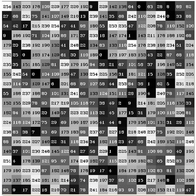
灰度值的取值范围在[0, 255]，每15个强度值划为一组，共得到16个子块

\[ [0,255]=[0,15]∪[16,31]∪....∪[240,255] \]

\[ range=bin_{1} ∪ bin_{2} ∪ .... ∪ bin_{n}=15 \]

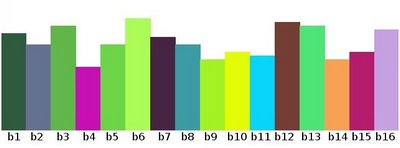
统计每个子块中的像素个数，得到的就是颜色直方图。图形化显示如下（x轴表示bin，y轴表示像素个数）

关键参数

直方图有3个关键参数：

dims：要收集数据的参数数量。在上式灰度图像中，仅收集每个像素的强度值（灰度值），所以dims=1
bins：每个dim中根据强度级别划分的子块数。上式中，灰度值取值范围在[0,255]，每15个强度值划为一组，共得到16个bin - bins=16
range：要测量的值的取值范围。上式中，要测量灰度值，取值为[0,255]

直方图的作用

它表示了图像强度分布
它量化了每个强度值的像素数

所以使用直方图能够统计数据的全局信息

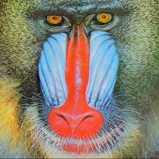
直方图计算

参考：calcHist() [1/3]

实现步骤如下：

加载图像
分离彩色图像到R/G/B通道
计算每个通道的颜色直方图
在同一图上绘制3个颜色直方图

OpenCV提供了cv::calcHist用于直方图计算

CV_EXPORTS void calcHist( const Mat* images, int nimages,
                          const int* channels, InputArray mask,
                          OutputArray hist, int dims, const int* histSize,
                          const float** ranges, bool uniform = true, bool accumulate = false );

images：原图数组。应该具有相同的深度（CV_8U、CV_16U或CV_32F）以及相同的尺寸。每个图像可以有任意数量的通道
nimages：图像个数
channels：用于计算直方图的dims通道列表。第一个列表值表示计算第一张图像的前几个通道；第二个列表值表示计算第二张图像的前几个通道，最后累加到一起得到直方图
mask：可选。如果矩阵不是空的，它必须是一个8位数组，大小与images[i]相同。非零掩码元素标记会被直方图计数的数组元素（比如仅计算图像中某一区域的直方图）
hist：输出直方图
dims：直方图维数，必须是正数，不大于CV_MAX_DIMS（当前取值为32）
histSize：每个维度的直方图大小数组
ranges：每个图像的取值范围
uniform：默认为true，表示每张图片计算的直方图是否一致
accumulate：累积标志。如果已设置，直方图在分配时不会在开始时被清除。此功能使您能够从几组数组中计算出一个直方图，或者及时更新直方图

示例如下：

#include "opencv2/highgui.hpp"
#include "opencv2/imgcodecs.hpp"
#include "opencv2/imgproc.hpp"
#include <iostream>
using namespace std;
using namespace cv;
int main(int argc, char** argv)
{
    CommandLineParser parser( argc, argv, "{@input | ../data/lena.jpg | input image}" );
    Mat src = imread( parser.get<String>( "@input" ), IMREAD_COLOR );
    if( src.empty() )
    {
        return -1;
    }
    vector<Mat> bgr_planes;
    split( src, bgr_planes );
    int histSize = 256;
    float range[] = { 0, 256 }; //the upper boundary is exclusive
    const float* histRange = { range };
    bool uniform = true, accumulate = false;
    Mat b_hist, g_hist, r_hist;
    calcHist( &bgr_planes[0], 1, 0, Mat(), b_hist, 1, &histSize, &histRange, uniform, accumulate );
    calcHist( &bgr_planes[1], 1, 0, Mat(), g_hist, 1, &histSize, &histRange, uniform, accumulate );
    calcHist( &bgr_planes[2], 1, 0, Mat(), r_hist, 1, &histSize, &histRange, uniform, accumulate );
    int hist_w = 512, hist_h = 400;
    int bin_w = cvRound( (double) hist_w/histSize );
    Mat histImage( hist_h, hist_w, CV_8UC3, Scalar( 0,0,0) );
    normalize(b_hist, b_hist, 0, histImage.rows, NORM_MINMAX, -1, Mat() );
    normalize(g_hist, g_hist, 0, histImage.rows, NORM_MINMAX, -1, Mat() );
    normalize(r_hist, r_hist, 0, histImage.rows, NORM_MINMAX, -1, Mat() );
    for( int i = 1; i < histSize; i++ )
    {
        line( histImage, Point( bin_w*(i-1), hist_h - cvRound(b_hist.at<float>(i-1)) ),
              Point( bin_w*(i), hist_h - cvRound(b_hist.at<float>(i)) ),
              Scalar( 255, 0, 0), 2, 8, 0  );
        line( histImage, Point( bin_w*(i-1), hist_h - cvRound(g_hist.at<float>(i-1)) ),
              Point( bin_w*(i), hist_h - cvRound(g_hist.at<float>(i)) ),
              Scalar( 0, 255, 0), 2, 8, 0  );
        line( histImage, Point( bin_w*(i-1), hist_h - cvRound(r_hist.at<float>(i-1)) ),
              Point( bin_w*(i), hist_h - cvRound(r_hist.at<float>(i)) ),
              Scalar( 0, 0, 255), 2, 8, 0  );
    }
    imshow("Source image", src );
    imshow("calcHist Demo", histImage );
    waitKey();
    return 0;
}

直方图均衡

参考：

Histogram equalization

直方图均衡化

直方图均衡通过扩展像素取值范围，能够提高图像对比度

均衡意味着将一个分布(给定直方图)映射到另一个分布(更宽和更均匀的分布)，以便强度值分布在整个范围内

操作步骤

第一步：统计灰度直方图

第二步：计算每一级灰度的概率

\[ p_{x}(i) = p(x=i) = \frac {n_{i}}{n}, 0\leq i < L \]

其中\(L\)表示灰度级数（通常为\(256\)），\(n\)表示图像像素个数，\(p_{x}(i)\)表示直方图中像素值为\(i\)的概率

第三步：计算累积分布函数cdf(cumulative distribution function)

\[ cdf_{x}(i) = \sum_{j=0}^{i}p_{x}(j) \]

第四步：求取映射像素值

\[ s_{i} = T(r_{i}) = round((L-1)*cdf_{x}(i) + 0.5) \]

函数\(T\)表示映射函数
函数\(round\)表示去除小数部分取整数
\((L-1)*cdf_{x}(i)\)表示将像素值扩展回原先的级数

经过第四步计算完成后就能够得到直方图均衡后的结果

OpenCV使用

OpenCV提供了函数equalizeHist()进行直方图均衡化的操作

1	CV_EXPORTS_W void equalizeHist( InputArray src, OutputArray dst );

参数src是一个8位单通道图像，输出dst得到和原图同样大小和类型的结果

...
Mat src = imread(parser.get<String>("@input"), IMREAD_COLOR);
if (src.empty()) {
    cout << "Could not open or find the image!\n" << endl;
    cout << "Usage: " << argv[0] << " <Input image>" << endl;
    return -1;
}
cvtColor(src, src, COLOR_BGR2GRAY);
Mat dst;
equalizeHist(src, dst);

imshow("Source image", src);
imshow("Equalized Image", dst);
waitKey();
...

直方图比较

参考：HistCompMethods

直方图比较的目的是计算两个直方图的匹配程度

OpenCV提供了四种比较方式

Correlation
Chi-Square
Intersection（直方图相交）
Bhattacharyya distance

直方图相交

计算公式如下：

\[ d(H_{1}, H_{2}) = \sum_{I} \min (H_{1}(I), H_{2}(I)) \]

\(H_{1}\)和\(H_{2}\)是两个直方图

操作步骤

参考：颜色直方图，HSV直方图

加载两张比较图像
转换成HSV格式，计算H-S直方图
使用直方图比较方式进行计算
输出匹配数值

将图像转换成HSV格式后再进行直方图比较，更能够符合人眼对颜色相似性的主观判断

OpenCV示例

...
    Mat src_base = imread(path);
    Mat src_test = imread(path2);
    if (src_base.empty() || src_test.empty()) {
        cout << "Could not open or find the images!\n" << endl;
        return -1;
    }

    Mat hsv_base, hsv_test1;
    cvtColor(src_base, hsv_base, COLOR_BGR2HSV);
    cvtColor(src_test, hsv_test1, COLOR_BGR2HSV);

    int h_bins = 50, s_bins = 60;
    int histSize[] = {h_bins, s_bins};
    // hue varies from 0 to 179, saturation from 0 to 255
    float h_ranges[] = {0, 180};
    float s_ranges[] = {0, 256};
    const float *ranges[] = {h_ranges, s_ranges};
    // Use the 0-th and 1-st channels
    int channels[] = {0, 1};

    Mat hist_base, hist_test;
    calcHist(&hsv_base, 1, channels, Mat(), hist_base, 2, histSize, ranges, true, false);
    normalize(hist_base, hist_base, 0, 1, NORM_MINMAX, -1, Mat());

    calcHist(&hsv_test1, 1, channels, Mat(), hist_test, 2, histSize, ranges, true, false);
    normalize(hist_test, hist_test, 0, 1, NORM_MINMAX, -1, Mat());

    double base_test = compareHist(hist_base, hist_test, HISTCMP_INTERSECT);
    cout << "Method HISTCMP_INTERSECT : " << base_test << endl;
...

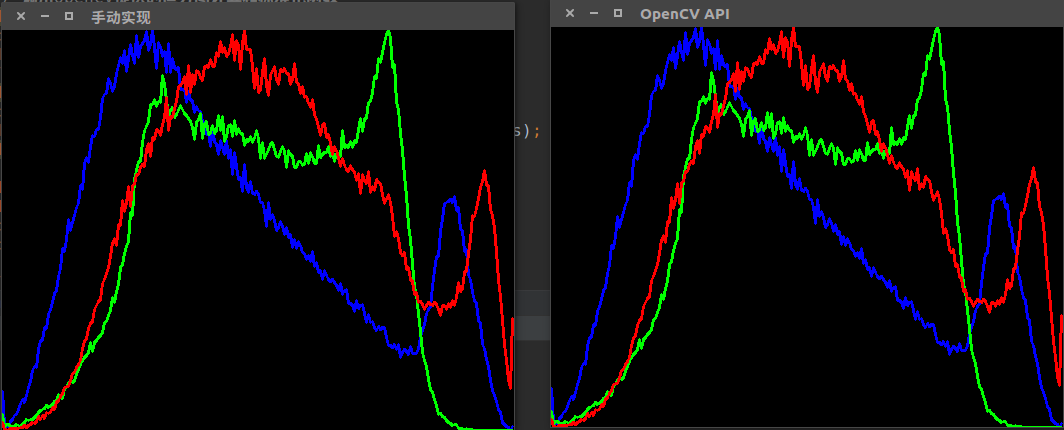
手动实现直方图计算

直方图计算主要涉及cv::calcHist和cv::normalize的使用。完整代码如下

//
// Created by zj on 19-11-24.
//

#include "opencv2/highgui.hpp"
#include "opencv2/imgcodecs.hpp"
#include "opencv2/imgproc.hpp"
#include <iostream>
#include <array>

using namespace std;
using namespace cv;

const static array<Scalar, 3> colors = {
        Scalar(255, 0, 0),
        Scalar(0, 255, 0),
        Scalar(0, 0, 255)
};

/**
 * 计算颜色直方图，图像取值固定为[0, 255]
 * @param src CV_8UC1或CV_8UC3大小图像
 * @param histograms 直方图向量
 * @param bins 直方图大小
 */
void calc_color_hist(const Mat &src, vector<Mat> &histograms, int bins) {
    int channels = src.channels();
    vector<Mat> img_planes;
    if (channels == 3) {
        split(src, img_planes);
    } else {
        // gray
        img_planes.emplace_back(src);
    }

    float range[] = {0, 256}; //the upper boundary is exclusive
    const float *histRange = {range};
    bool uniform = true, accumulate = false;

    for (int i = 0; i < channels; i++) {
        Mat hist;
        calcHist(&img_planes[i], 1, nullptr, Mat(), hist, 1, &bins, &histRange, uniform, accumulate);
//        cout << hist.type() << endl;
        histograms.emplace_back(hist);
    }
}

/**
 * 绘制直方图，首先对直方图标准化，再按比例绘制线条
 */
void draw_color_hist(const vector<Mat> &histograms, Mat &histImage, int bins) {
    int hist_w = 512, hist_h = 400;
    histImage = Mat(hist_h, hist_w, CV_8UC3, Scalar(0, 0, 0));

    int bin_w = cvRound((double) hist_w / bins);
    for (int i = 0; i < histograms.size(); i++) {
        Mat hist = histograms[i];
        Mat hist_tmp;
        // 标准化直方图，取值为[0.0, hist_h]
        normalize(hist, hist_tmp, 0, histImage.rows, NORM_MINMAX, -1, Mat());
//        cout << hist_tmp.type() << endl;
        Scalar color = colors[i % colors.size()];
        for (int i = 1; i < bins; i++) {
            line(histImage,
                 Point(bin_w * (i - 1), hist_h - cvRound(hist_tmp.at<float>(i - 1))),
                 Point(bin_w * (i), hist_h - cvRound(hist_tmp.at<float>(i))),
                 color,
                 2, 8, 0);
        }
    }
}

/**
 * 手动计算颜色直方图
 * @param src CV_8UC1或CV_8UC3
 * @param histograms 颜色直方图向量
 * @param bins 直方图大小
 */
void calc_color_hist_manully(const Mat &src, vector<Mat> &histograms, int bins) {
    int channels = src.channels();
    float ranges[] = {0.0, 256.0};
    // 计算每个bin的取值范围
    double range = (ranges[1] - ranges[0]) / bins;

    // 分离图像
    vector<Mat> img_planes;
    if (channels == 1) {
        img_planes.emplace_back(src);
    } else {
        // 分离3通道
        split(src, img_planes);
    }

    // 遍历所有通道，计算颜色直方图
    for (int i = 0; i < channels; i++) {
        Mat hist = Mat::zeros(1, bins, CV_32F);
        auto *hdata = hist.ptr<float>(0);

        Mat plane = img_planes[i];
        // 遍历所有像素，从左到右，从上到下
        for (int y = 0; y < plane.rows; y++) {
            auto *pdata = plane.ptr<uchar>(y);

            for (int x = 0; x < plane.cols; x++) {
                hdata[cvFloor(static_cast<int>(pdata[x]) / range)] += 1;
            }
        }
        histograms.emplace_back(hist);
    }
}

/**
 * 绘制直方图，首先手动对直方图标准化，再按比例绘制线条
 * @param histograms 直方图列表
 * @param histImage 绘制直方图
 * @param bins 直方图大小
 */
void draw_color_hist_manully(const vector<Mat> &histograms, Mat &histImage, int bins) {
    int hist_w = 512, hist_h = 400;
    histImage = Mat(hist_h, hist_w, CV_8UC3, Scalar(0, 0, 0));

    auto channels = histograms.size();

    // 手动标准化直方图
    vector<Mat> hist_tmps;
    for (int i = 0; i < channels; i++) {
        double min, max;
        cv::minMaxLoc(histograms[i], &min, &max);
        Mat hist_tmp = Mat::zeros(histograms[i].size(), CV_32F);

        auto *hdata = histograms[i].ptr<float>(0);
        auto *hdata_tmp = hist_tmp.ptr<float>(0);
        for (int j = 0; j < bins; j++) {
            hdata_tmp[j] = static_cast<float>(hist_h * (hdata[j] - min) / (max - min));
        }
        hist_tmps.emplace_back(hist_tmp);
    }

    int bin_w = cvRound(1.0 * hist_w / bins);
    for (int i = 0; i < channels; i++) {
        Scalar color = colors[i % colors.size()];
        auto *hdata = hist_tmps[i].ptr<float>(0);

        for (int j = 1; j < bins; j++) {
            line(histImage,
                 Point(bin_w * (j - 1), cvRound(hist_h - hdata[j - 1])),
                 Point(bin_w * (j), cvRound(hist_h - hdata[j])),
                 color,
                 2, 8, 0);
        }
    }
}

int main(int argc, char **argv) {
    CommandLineParser parser(argc, argv, "{@input | ../lena.jpg | input image}");
    Mat src = imread(parser.get<String>("@input"), IMREAD_COLOR);
    if (src.empty()) {
        return -1;
    }

//    Mat gray;
//    cvtColor(src, gray, COLOR_BGR2GRAY);
//    src = gray;

    int bins = 256;
    vector<Mat> histograms, histograms2;
    Mat histImage, histImage2;

    // 调用OpenCV提供的直方图计算和标准化函数
    double t1 = (double) getTickCount();
    calc_color_hist(src, histograms, bins);
    draw_color_hist(histograms, histImage, bins);
    // 手动计算和标准化直方图
    double t2 = (double) getTickCount();
    calc_color_hist_manully(src, histograms2, bins);
    draw_color_hist_manully(histograms2, histImage2, bins);
    double t3 = (double) getTickCount();

    double time1 = (t2 - t1) / getTickFrequency();
    double time2 = (t3 - t2) / getTickFrequency();
    cout << time1 << endl;
    cout << time2 << endl;

    // 判断绘制图像是否相等
    cv::Mat diff = histImage != histImage2;
    cout << sum(diff) << endl;

    imshow("Source image", src);
    imshow("OpenCV API", histImage);
    imshow("手动实现", histImage2);
    waitKey();

    return 0;
}