softmax回归

softmax回归常用于多分类问题,其输出可直接看成对类别的预测概率

假设对k类标签([1, 2, ..., k])进行分类,那么经过softmax回归计算后,输出一个k维向量,向量中每个值都代表对一个类别的预测概率

下面先以单个输入数据为例,进行评分函数、损失函数的计算和求导,然后扩展到多个输入数据同步计算

对数函数操作

对数求和

\[ log_{a}^{x}+log_{a}^{y} = log_{a}^{xy} \]

对数求差

\[ log_{a}^{x}-log_{a}^{y} = log_{a}^{\frac{x}{y}} \]

指数乘法

\[ e^{x}\cdot e^{y} = e^{x+y} \]

求导公式

若函数\(u(x),v(x)均可导\),那么

\[ \left(\frac{u(x)}{v(x)}\right)^{\prime}=\frac{u^{\prime}(x) v(x)-v^{\prime}(x) u(x)}{v^{2}(x)} \]

单个输入数据进行softmax回归计算

评分函数

假设使用softmax回归分类数据\(x\),共\(k\)个标签,首先进行线性回归操作

\[ z_{\theta}(x)=\theta^T\cdot x =\begin{bmatrix} \theta_{1}^T\\ \theta_{2}^T\\ ...\\ \theta_{k}^T \end{bmatrix}\cdot x =\begin{bmatrix} \theta_{1}^T\cdot x\\ \theta_{2}^T\cdot x\\ ...\\ \theta_{k}^T\cdot x \end{bmatrix} \]

其中输入数据\(x\)大小为\((n+1)\times 1\)\(\theta\)大小为\((n+1)\times k\)\(n\)表示权重数量,\(m\)表示训练数据个数,\(k\)表示类别标签数量

输出结果\(z\)大小为\(k\times 1\),然后对计算结果进行归一化操作,使得输出值能够表示类别概率,如下所示

\[ h_{\theta}\left(x\right)=\left[ \begin{array}{c}{p\left(y=1 | x ; \theta\right)} \\ {p\left(y=2 | x ; \theta\right)} \\ {\vdots} \\ {p\left(y=k | x ; \theta\right)}\end{array}\right] =\frac{1}{\sum_{j=1}^{k} e^{\theta_{j}^{T} x}} \left[ \begin{array}{c}{e^{\theta_{1}^{T} x}} \\ {e^{\theta_{2}^{T} x}} \\ {\vdots} \\ {e^{\theta_{k}^{T} x}}\end{array}\right] \]

其中\(\theta_{1}、\theta_{2},...,\theta_{k}\)的大小为\((n+1)\times 1\),输出结果是一个\(k\times 1\)大小向量,每列表示\(k\)类标签的预测概率

所以对于输入数据\(x\)而言,其属于标签\(j\)的概率是

\[ p\left(y=j | x; \theta\right)=\frac{e^{\theta_{j}^{T} x}}{\sum_{l=1}^{k} e^{\theta_{l}^{T} x}} \]

损失函数

利用交叉熵损失(cross entropy loss)作为softmax回归的损失函数,用于计算训练数据对应的真正标签的损失值

\[ J(\theta) = (-1)\cdot \sum_{j=1}^{k} 1\left\{y=j\right\} \ln p\left(y=j | x; \theta\right) = (-1)\cdot \sum_{j=1}^{k} 1\left\{y=j\right\} \ln \frac{e^{\theta_{j}^{T} x}}{\sum_{l=1}^{k} e^{\theta_{l}^{T} x}} \]

其中函数\(1\{\cdot\}\)是一个示性函数(indicator function),其取值规则为

1
1{a true statement} = 1, and 1{a false statement} = 0

也就是示性函数输入为True时,输出为1;否则,输出为0

对权重向量\(\theta_{s}\)进行求导:

\[ \frac{\varphi J(\theta)}{\varphi \theta_{s}} =(-1)\cdot \frac{\varphi }{\varphi \theta_{s}} \left[ \\ \sum_{j=1,j\neq s}^{k} 1\left\{y=j \right\} \ln p\left(y=j | x; \theta\right) +1\left\{y=s \right\} \ln p\left(y=s | x; \theta\right) \\ \right] \]

\[ =(-1)\cdot \sum_{j=1,j\neq s}^{k} 1\left\{y=j \right\} \frac{1}{p\left(y=j | x; \theta\right)}\frac{\varphi p\left(y=j | x; \theta\right)}{\varphi \theta_{s}} +(-1)\cdot 1\left\{y=s \right\} \frac{1}{p\left(y=s | x; \theta\right)}\frac{\varphi p\left(y=s | x; \theta\right)}{\varphi \theta_{s}} \]

分为两种情况

  • 当计算结果正好由\(\theta_{s}\)计算得到,此时线性运算为\(z=\theta_{s}^{T} x\),计算结果为\(p\left(y=s | x; \theta\right)=\frac{e^{\theta_{s}^{T} x}}{\sum_{l=1}^{k} e^{\theta_{l}^{T} x}}\),求导如下

\[ \frac{\varphi p\left(y=s | x; \theta\right)}{\varphi \theta_{s}} =\frac{u^{\prime}(x) v(x)-v^{\prime}(x) u(x)}{v^{2}(x)} \]

其中

\[ u(x) = e^{\theta_{s}^{T} x}, v(x)=\sum_{l=1}^{k} e^{\theta_{l}^{T} x} \]

所以

\[ \frac{\varphi u(x)}{\varphi \theta_s} = e^{\theta_{s}^{T} x}\cdot x=u(x)\cdot x, \frac{\varphi v(x)}{\varphi \theta_s} = e^{\theta_{s}^{T} x}\cdot x=u(x)\cdot x \\ \frac{\varphi p\left(y=s | x; \theta\right)}{\varphi \theta_{s}} = p\left(y=s | x; \theta\right)\cdot x-p\left(y=s | x; \theta\right)^2\cdot x \]

  • 当计算结果不是由\(\theta_{s}\)计算得到,此时线性运算为\(z=\theta_{j}^{T} x, j\neq s\),计算结果为\(p\left(y=j | x; \theta\right)=\frac{e^{\theta_{j}^{T} x}}{\sum_{l=1}^{k} e^{\theta_{l}^{T} x}}\)

\[ \frac{\varphi p\left(y=j | x; \theta\right)}{\varphi \theta_{s}} =\frac{u^{\prime}(x) v(x)-v^{\prime}(x) u(x)}{v^{2}(x)} \]

其中

\[ u(x) = e^{\theta_{j}^{T} x}, v(x)=\sum_{l=1}^{k} e^{\theta_{l}^{T} x} \]

所以

\[ \frac{\varphi u(x)}{\varphi \theta_s} = e^{\theta_{j}^{T} x}\cdot x=0, \frac{\varphi v(x)}{\varphi \theta_s} = e^{\theta_{s}^{T} x}\cdot x \\ \frac{\varphi p\left(y=s | x; \theta\right)}{\varphi \theta_{s}} = -p\left(y=s | x; \theta\right)p\left(y=j | x; \theta\right)\cdot x \]

综合上述两种情况可知,求导结果为

\[ \frac{\varphi J(\theta)}{\varphi \theta_{s}} =(-1)\cdot \sum_{j=1,j\neq s}^{k} 1\left\{y=j \right\} \frac{1}{p\left(y=j | x; \theta\right)}\frac{\varphi p\left(y=j | x; \theta\right)}{\varphi \theta_{s}} +(-1)\cdot 1\left\{y=s \right\} \frac{1}{p\left(y=s | x; \theta\right)}\frac{\varphi p\left(y=s | x; \theta\right)}{\varphi \theta_{s}} \\ =(-1)\cdot \sum_{j=1,j\neq s}^{k} 1\left\{y=j \right\} \frac{1}{p\left(y=j | x; \theta\right)})\cdot (-1)\cdot p\left(y=s | x; \theta\right)p\left(y=j | x; \theta\right)\cdot x + (-1)\cdot 1\left\{y=s \right\} \frac{1}{p\left(y=s | x; \theta\right)}\left[p\left(y=s | x; \theta\right)\cdot x-p\left(y=s | x; \theta\right)^2\cdot x\right] \\ =(-1)\cdot \sum_{j=1,j\neq s}^{k} 1\left\{y=j \right\}\cdot (-1)\cdot p\left(y=s | x; \theta\right)\cdot x + (-1)\cdot 1\left\{y=s \right\} \left[x-p\left(y=s | x; \theta\right)\cdot x\right] \\ =(-1)\cdot 1\left\{y=s \right\} x - (-1)\cdot \sum_{j=1}^{k} 1\left\{y=j \right\} p\left(y=s | x; \theta\right)\cdot x \]

因为\(\sum_{j=1}^{k} 1\left\{y=j \right\}=1\),所以最终结果为

\[ \frac{\varphi J(\theta)}{\varphi \theta_{s}} =(-1)\cdot \left[ 1\left\{y=s \right\} - p\left(y=s | x; \theta\right) \right]\cdot x \]

批量数据进行softmax回归计算

上面实现了单个数据进行类别概率和损失函数的计算以及求导,进一步推导到批量数据进行操作

评分函数

假设使用softmax回归分类数据\(x\),共\(k\)个标签,首先进行线性回归操作

\[ z_{\theta}(x_{i})=\theta^T\cdot x_{i} =\begin{bmatrix} \theta_{1}^T\\ \theta_{2}^T\\ ...\\ \theta_{k}^T \end{bmatrix}\cdot x_{i} =\begin{bmatrix} \theta_{1}^T\cdot x_{i}\\ \theta_{2}^T\cdot x_{i}\\ ...\\ \theta_{k}^T\cdot x_{i} \end{bmatrix} \]

其中输入数据\(x\)大小为\((n+1)\times m\)\(\theta\)大小为\((n+1)\times k\)\(n\)表示权重数量,\(m\)表示训练数据个数,\(k\)表示类别标签数量

输出结果\(z\)大小为\(k\times m\),然后对计算结果进行归一化操作,使得输出值能够表示类别概率,如下所示

\[ h_{\theta}\left(x_{i}\right)=\left[ \begin{array}{c}{p\left(y=1 | x_{i} ; \theta\right)} \\ {p\left(y=2 | x_{i} ; \theta\right)} \\ {\vdots} \\ {p\left(y=k | x_{i} ; \theta\right)}\end{array}\right] =\frac{1}{\sum_{j=1}^{k} e^{\theta_{j}^{T} x}} \left[ \begin{array}{c}{e^{\theta_{1}^{T} x_{i}}} \\ {e^{\theta_{2}^{T} x_{i}}} \\ {\vdots} \\ {e^{\theta_{k}^{T} x_{i}}}\end{array}\right] \]

其中\(\theta_{1}、\theta_{2},...,\theta_{k}\)的大小为\((n+1)\times 1\),输出结果是一个\(k\times m\)大小向量,每列表示\(k\)类标签的预测概率

所以对于输入数据\(x_{i}\)而言,其属于标签\(j\)的概率是

\[ p\left(y_{i}=j | x_{i}; \theta\right)=\frac{e^{\theta_{j}^{T} x_{i}}}{\sum_{l=1}^{k} e^{\theta_{l}^{T} x_{i}}} \]

代价函数

利用交叉熵损失(cross entropy loss)作为softmax回归的代价函数,用于计算训练数据对应的真正标签的损失值

\[ J(\theta) = (-1)\cdot \frac{1}{m}\cdot \sum_{i=1}^{m} \sum_{j=1}^{k} 1\left\{y_{i}=j\right\} \ln p\left(y_{i}=j | x_{i}; \theta\right) = (-1)\cdot \frac{1}{m}\cdot \sum_{i=1}^{m} \sum_{j=1}^{k} 1\left\{y_{i}=j\right\} \ln \frac{e^{\theta_{j}^{T} x_{i}}}{\sum_{l=1}^{k} e^{\theta_{l}^{T} x_{i}}} \]

其中函数\(1\{\cdot\}\)是一个示性函数(indicator function),其取值规则为

1
1{a true statement} = 1, and 1{a false statement} = 0

也就是示性函数输入为True时,输出为1;否则,输出为0

对权重向量\(\theta_{s}\)进行求导:

\[ \frac{\varphi J(\theta)}{\varphi \theta_{s}} =(-1)\cdot \frac{1}{m}\cdot \sum_{i=1}^{m}\cdot \frac{\varphi }{\varphi \theta_{s}} \left[ \sum_{j=1,j\neq s}^{k} 1\left\{y_{i}=j \right\} \ln p\left(y_{i}=j | x_{i}; \theta\right)+1\left\{y_{i}=s \right\} \ln p\left(y_{i}=s | x_{i}; \theta\right) \right] \]

\[ =(-1)\cdot \frac{1}{m}\cdot \sum_{i=1}^{m}\cdot \sum_{j=1,j\neq s}^{k} 1\left\{y_{i}=j \right\} \frac{1}{p\left(y_{i}=j | x_{i}; \theta\right)}\frac{\varphi p\left(y_{i}=j | x_{i}; \theta\right)}{\varphi \theta_{s}} +(-1)\cdot \frac{1}{m}\cdot \sum_{i=1}^{m}\cdot 1\left\{y_{i}=s \right\} \frac{1}{p\left(y_{i}=s | x_{i}; \theta\right)}\frac{\varphi p\left(y_{i}=s | x_{i}; \theta\right)}{\varphi \theta_{s}} \]

分为两种情况

  • 当计算结果正好由\(\theta_{s}\)计算得到,此时线性运算为\(z=\theta_{s}^{T} x_{i}\),计算结果为\(p\left(y_{i}=s | x_{i}; \theta\right)=\frac{e^{\theta_{s}^{T} x_{i}}}{\sum_{l=1}^{k} e^{\theta_{l}^{T} x_{i}}}\),求导如下

\[ \frac{\varphi p\left(y_{i}=s | x_{i}; \theta\right)}{\varphi \theta_{s}} =\frac{u^{\prime}(x) v(x)-v^{\prime}(x) u(x)}{v^{2}(x)} \]

其中

\[ u(x) = e^{\theta_{s}^{T} x}, v(x)=\sum_{l=1}^{k} e^{\theta_{l}^{T} x} \]

所以

\[ \frac{\varphi u(x)}{\varphi \theta_s} = e^{\theta_{s}^{T} x}\cdot x=u(x)\cdot x, \frac{\varphi v(x)}{\varphi \theta_s} = e^{\theta_{s}^{T} x}\cdot x=u(x)\cdot x \\ \frac{\varphi p\left(y=s | x_{i}; \theta\right)}{\varphi \theta_{s}} = p\left(y=s | x_{i}; \theta\right)\cdot x_{i}-p\left(y=s | x_{i}; \theta\right)^2\cdot x_{i} \]

  • 当计算结果不是由\(\theta_{s}\)计算得到,此时线性运算为\(z=\theta_{j}^{T} x_{i}, j\neq s\),计算结果为\(p\left(y_{i}=j | x_{i}; \theta\right)=\frac{e^{\theta_{j}^{T} x_{i}}}{\sum_{l=1}^{k} e^{\theta_{l}^{T} x_{i}}}\)

\[ \frac{\varphi p\left(y_{i}=j | x_{i}; \theta\right)}{\varphi \theta_{s}} =\frac{u^{\prime}(x) v(x)-v^{\prime}(x) u(x)}{v^{2}(x)} \]

其中

\[ u(x) = e^{\theta_{j}^{T} x}, v(x)=\sum_{l=1}^{k} e^{\theta_{l}^{T} x} \]

所以

\[ \frac{\varphi u(x)}{\varphi \theta_s} = e^{\theta_{j}^{T} x}\cdot x=0, \frac{\varphi v(x)}{\varphi \theta_s} = e^{\theta_{s}^{T} x}\cdot x \\ \frac{\varphi p\left(y_{i}=s | x_{i}; \theta\right)}{\varphi \theta_{s}} = -p\left(y_{i}=s | x_{i}; \theta\right)p\left(y_{i}=j | x_{i}; \theta\right)\cdot x_{i} \]

综合上述两种情况可知,求导结果为

\[ \frac{\varphi J(\theta)}{\varphi \theta_{s}} =(-1)\cdot \frac{1}{m}\cdot \sum_{i=1}^{m}\cdot \sum_{j=1,j\neq s}^{k} 1\left\{y_{i}=j \right\} \frac{1}{p\left(y_{i}=j | x_{i}; \theta\right)}\frac{\varphi p\left(y_{i}=j | x_{i}; \theta\right)}{\varphi \theta_{s}} +(-1)\cdot \frac{1}{m}\cdot \sum_{i=1}^{m}\cdot 1\left\{y_{i}=s \right\} \frac{1}{p\left(y_{i}=s | x_{i}; \theta\right)}\frac{\varphi p\left(y_{i}=s | x_{i}; \theta\right)}{\varphi \theta_{s}} \\ =(-1)\cdot \frac{1}{m}\cdot \sum_{i=1}^{m}\cdot \sum_{j=1,j\neq s}^{k} 1\left\{y_{i}=j \right\} \frac{1}{p\left(y_{i}=j | x_{i}; \theta\right)})\cdot (-1)\cdot p\left(y_{i}=s | x_{i}; \theta\right)p\left(y_{i}=j | x_{i}; \theta\right)\cdot x_{i} + (-1)\cdot \frac{1}{m}\cdot \sum_{i=1}^{m}\cdot 1\left\{y_{i}=s \right\} \frac{1}{p\left(y_{i}=s | x_{i}; \theta\right)}\left[p\left(y_{i}=s | x_{i}; \theta\right)\cdot x_{i}-p\left(y_{i}=s | x_{i}; \theta\right)^2\cdot x_{i}\right] \\ =(-1)\cdot \frac{1}{m}\cdot \sum_{i=1}^{m}\cdot \sum_{j=1,j\neq s}^{k} 1\left\{y_{i}=j \right\}\cdot (-1)\cdot p\left(y_{i}=s | x_{i}; \theta\right)\cdot x_{i} + (-1)\cdot \frac{1}{m}\cdot \sum_{i=1}^{m}\cdot 1\left\{y_{i}=s \right\} \left[x_{i}-p\left(y_{i}=s | x_{i}; \theta\right)\cdot x_{i}\right] \\ =(-1)\cdot \frac{1}{m}\cdot \sum_{i=1}^{m}\cdot 1\left\{y_{i}=s \right\} x_{i} - (-1)\cdot \frac{1}{m}\cdot \sum_{i=1}^{m}\cdot \sum_{j=1}^{k} 1\left\{y_{i}=j \right\} p\left(y_{i}=s | x_{i}; \theta\right)\cdot x_{i} \]

因为\(\sum_{j=1}^{k} 1\left\{y_{i}=j \right\}=1\),所以最终结果为

\[ \frac{\varphi J(\theta)}{\varphi \theta_{s}} =(-1)\cdot \frac{1}{m}\cdot \sum_{i=1}^{m}\cdot \left[ 1\left\{y_{i}=s \right\} - p\left(y_{i}=s | x_{i}; \theta\right) \right]\cdot x_{i} \]

梯度下降

权重\(W\)大小为\((n+1)\times k\),输入数据集大小为\(m\times (n+1)\),输出数据集大小为\(m\times k\)

矩阵求导如下:

\[ \frac{\varphi J(\theta)}{\varphi \theta} =\frac{1}{m}\cdot \sum_{i=1}^{m}\cdot \begin{bmatrix} (-1)\cdot\left[ 1\left\{y=1 \right\} - p\left(y=1 | x; \theta\right) \right]\cdot x\\ (-1)\cdot\left[ 1\left\{y=2 \right\} - p\left(y=2 | x; \theta\right) \right]\cdot x\\ ...\\ (-1)\cdot\left[ 1\left\{y=k \right\} - p\left(y=k | x; \theta\right) \right]\cdot x \end{bmatrix} =(-1)\cdot \frac{1}{m}\cdot X_{m\times n+1}^T \cdot (I_{m\times k} - Y_{m\times k}) \]

参考:

Softmax regression for Iris classification

Derivative of Softmax loss function

上述计算的是输入单个数据时的评分、损失和求导,所以使用随机梯度下降法进行权重更新,分类

参数冗余和权重衰减

softmax回归存在参数冗余现象,即对参数向量\(\theta_{j}\)减去向量$$不改变预测结果。证明如下:

\[ \begin{aligned} p\left(y^{(i)}=j | x^{(i)} ; \theta\right) &=\frac{e^{\left(\theta_{j}-\psi\right)^{T} x^{(i)}}}{\sum_{l=1}^{k} e^{\left(\theta_{l}-\psi\right)^{T} x^{(i)}}} \\ &=\frac{e^{\theta_{j}^{T} x^{(i)}} e^{-\psi^{T} x^{(i)}}}{\sum_{l=1}^{k} e^{\theta_{l}^{T} x^{(i)}} e^{-\psi^{T} x^{(i)}}} \\ &=\frac{e^{\theta_{j}^{T} x^{(i)}}}{\sum_{l=1}^{k} e^{\theta_{t}^{T} x^{(i)}}} \end{aligned} \]

假设\((\theta_{1},\theta_{2},...,\theta_{k})\)能得到\(j(\theta)\)的极小值点,那么\((\theta_{1}-\varphi,\theta_{2}-\varphi,...,\theta_{k}-\varphi)\)同样能得到相同的极小值点

与此同时,因为损失函数是凸函数,局部最小值就是全局最小值,所以会导致权重在参数过大情况下就停止收敛,影响模型泛化能力

在代价函数中加入权重衰减,能够避免过度参数化,得到泛化性能更强的模型

在代价函数中加入L2正则化项,如下所示:

\[ J(\theta) = (-1)\cdot \frac{1}{m}\cdot \sum_{i=1}^{m} \sum_{j=1}^{k} 1\left\{y_{i}=j\right\} \ln p\left(y_{i}=j | x_{i}; \theta\right) + \frac{\lambda}{2} \sum_{i=1}^{k} \sum_{j=0}^{n} \theta_{i j}^{2} = (-1)\cdot \frac{1}{m}\cdot \sum_{i=1}^{m} \sum_{j=1}^{k} 1\left\{y_{i}=j\right\} \ln \frac{e^{\theta_{j}^{T} x_{i}}}{\sum_{l=1}^{k} e^{\theta_{l}^{T} x_{i}}} + \frac{\lambda}{2} \sum_{i=1}^{k} \sum_{j=0}^{n} \theta_{i j}^{2} \]

求导结果如下:

\[ \frac{\varphi J(\theta)}{\varphi \theta_{s}} =(-1)\cdot \frac{1}{m}\cdot \sum_{i=1}^{m}\cdot \left[ 1\left\{y_{i}=s \right\} - p\left(y_{i}=s | x_{i}; \theta\right) \right]\cdot x_{i}+ \lambda \theta_{j} \]

代价实现如下:

1
2
3
4
5
6
7
8
9
10
11
12
13
14
15
16
17
18
19
20
21
def compute_loss(scores, indicator, W):
"""
计算损失值
:param scores: 大小为(m, n)
:param indicator: 大小为(m, n)
:param W: (n, k)
:return: (m,1)
"""
return -1 * np.sum(np.log(scores) * indicator, axis=1) + 0.001/2*np.sum(W**2)


def compute_gradient(indicator, scores, x, W):
"""
计算梯度
:param indicator: 大小为(m,k)
:param scores: 大小为(m,k)
:param x: 大小为(m,n)
:param W: (n, k)
:return: (n,k)
"""
return -1 * x.T.dot((indicator - scores)) + 0.001*W

鸢尾数据集

使用鸢尾(iris)数据集,参考Iris Species

4个变量:

  • SepalLengthCm - 花萼长度
  • SepalWidthCm - 花萼宽度
  • PetalLengthCm - 花瓣长度
  • PetalWidthCm - 花瓣宽度

以及3个类别:

  • Iris-setosa
  • Iris-versicolor
  • Iris-virginica
1
2
3
4
5
6
7
8
9
10
11
12
13
14
15
16
17
18
19
20
21
22
23
24
25
26
27
28
29
30
31
32
33
34
35
36
37
def load_data(shuffle=True, tsize=0.8):
"""
加载iris数据
"""
data = pd.read_csv(data_path, header=0, delimiter=',')
# print(data.columns)

draw_data(data.values, data.columns)

def draw_data(data, columns):
data_a = data[:50, 1:5]
data_b = data[50:100, 1:5]
data_c = data[100:150, 1:5]

fig = plt.figure(1)
plt.scatter(data_a[:, 0], data_a[:, 1], c='b', marker='8')
plt.scatter(data_b[:, 0], data_b[:, 1], c='r', marker='s')
plt.scatter(data_c[:, 0], data_c[:, 1], c='y', marker='*')
plt.xlabel(columns[1])
plt.ylabel(columns[2])
plt.show()

fig = plt.figure(2)
plt.scatter(data_a[:, 2], data_a[:, 3], c='b', marker='8')
plt.scatter(data_b[:, 2], data_b[:, 3], c='r', marker='s')
plt.scatter(data_c[:, 2], data_c[:, 3], c='y', marker='*')
plt.xlabel(columns[3])
plt.ylabel(columns[4])
plt.show()

# 验证是否有重复数据
# for i in range(data_b.shape[0]):
# res = list(filter(lambda x: x[0] == data_b[i][0] and x[1] == data_b[i][1], data_c[:, :2]))
# if len(res) != 0:
# res2 = list(filter(lambda x: x[2] == data_b[i][2] and x[3] == data_b[i][3], data_c[:, 2:4]))
# if len(res2) != 0:
# print(b[i])

numpy实现

1
2
3
4
5
6
7
8
9
10
11
12
13
14
15
16
17
18
19
20
21
22
23
24
25
26
27
28
29
30
31
32
33
34
35
36
37
38
39
40
41
42
43
44
45
46
47
48
49
50
51
52
53
54
55
56
57
58
59
60
61
62
63
64
65
66
67
68
69
70
71
72
73
74
75
76
77
78
79
80
81
82
83
84
85
86
87
88
89
90
91
92
93
94
95
96
97
98
99
100
101
102
103
104
105
106
107
108
109
110
111
112
113
114
115
116
117
118
119
120
121
122
123
124
125
126
127
128
129
130
131
132
133
134
135
136
137
138
139
140
141
142
143
144
145
146
147
148
149
150
151
152
153
154
155
156
157
158
159
160
161
162
163
164
165
166
167
168
169
170
171
172
173
174
175
176
# -*- coding: utf-8 -*-

# @Time : 19-4-25 上午10:30
# @Author : zj

import numpy as np
import matplotlib.pyplot as plt
import pandas as pd
from sklearn import utils
from sklearn.model_selection import train_test_split
import warnings

warnings.filterwarnings('ignore')

data_path = '../data/iris-species/Iris.csv'


def load_data(shuffle=True, tsize=0.8):
"""
加载iris数据
"""
data = pd.read_csv(data_path, header=0, delimiter=',')

if shuffle:
data = utils.shuffle(data)

# 示性函数
pd_indicator = pd.get_dummies(data['Species'])
indicator = np.array(
[pd_indicator['Iris-setosa'], pd_indicator['Iris-versicolor'], pd_indicator['Iris-virginica']]).T

species_dict = {
'Iris-setosa': 0,
'Iris-versicolor': 1,
'Iris-virginica': 2
}
data['Species'] = data['Species'].map(species_dict)

data_x = np.array(
[data['SepalLengthCm'], data['SepalWidthCm'], data['PetalLengthCm'], data['PetalWidthCm']]).T
data_y = data['Species']

x_train, x_test, y_train, y_test = train_test_split(data_x, data_y, train_size=tsize, test_size=(1 - tsize),
shuffle=False)

y_train = np.atleast_2d(y_train).T
y_test = np.atleast_2d(y_test).T

y_train_indicator = np.atleast_2d(indicator[:y_train.shape[0]])
y_test_indicator = indicator[y_train.shape[0]:]

return x_train, x_test, y_train, y_test, y_train_indicator, y_test_indicator


def linear(x, w):
"""
线性操作
:param x: 大小为(m,n+1)
:param w: 大小为(n+1,k)
:return: 大小为(m,k)
"""
return x.dot(w)


def softmax(x):
"""
softmax归一化计算
:param x: 大小为(m, k)
:return: 大小为(m, k)
"""
x -= np.atleast_2d(np.max(x, axis=1)).T
exps = np.exp(x)
return exps / np.atleast_2d(np.sum(exps, axis=1)).T


def compute_scores(X, W):
"""
计算精度
:param X: 大小为(m,n+1)
:param W: 大小为(n+1,k)
:return: (m,k)
"""
return softmax(linear(X, W))


def compute_loss(scores, indicator, W, la=2e-4):
"""
计算损失值
:param scores: 大小为(m, k)
:param indicator: 大小为(m, k)
:param W: (n+1, k)
:return: (1)
"""
cost = -1 / scores.shape[0] * np.sum(np.log(scores) * indicator)
reg = la / 2 * np.sum(W ** 2)
return cost + reg


def compute_gradient(scores, indicator, x, W, la=2e-4):
"""
计算梯度
:param scores: 大小为(m,k)
:param indicator: 大小为(m,k)
:param x: 大小为(m,n+1)
:param W: (n+1, k)
:return: (n+1,k)
"""
return -1 / scores.shape[0] * x.T.dot((indicator - scores)) + la * W


def compute_accuracy(scores, Y):
"""
计算精度
:param scores: (m,k)
:param Y: (m,1)
"""
res = np.dstack((np.argmax(scores, axis=1), Y.squeeze())).squeeze()

return len(list(filter(lambda x: x[0] == x[1], res[:]))) / len(res)


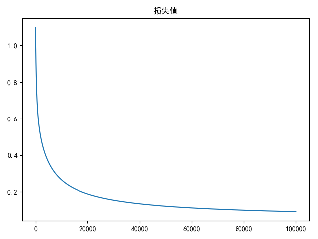
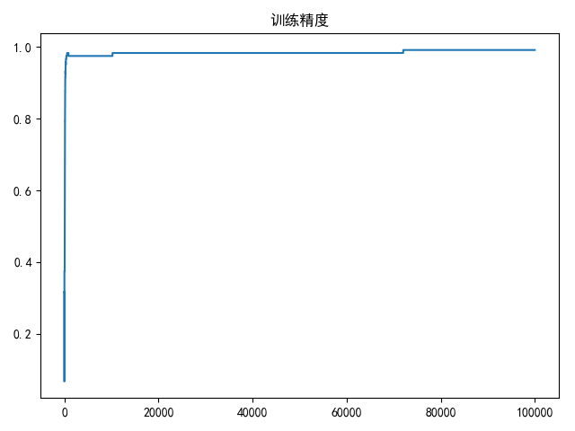
def draw(res_list, title=None, xlabel=None):
if title is not None:
plt.title(title)
if xlabel is not None:
plt.xlabel(xlabel)
plt.plot(res_list)
plt.show()


def compute_gradient_descent(batch_size=8, epoches=2000, alpha=2e-4):
x_train, x_test, y_train, y_test, y_train_indicator, y_test_indicator = load_data()

m, n = x_train.shape[:2]
k = y_train_indicator.shape[1]
# 初始化权重(n+1,k)
W = 0.01 * np.random.normal(loc=0.0, scale=1.0, size=(n + 1, k))
x_train = np.insert(x_train, 0, np.ones(m), axis=1)
x_test = np.insert(x_test, 0, np.ones(x_test.shape[0]), axis=1)

loss_list = []
accuracy_list = []
bestW = None
bestA = 0
range_list = np.arange(0, x_train.shape[0] - batch_size, step=batch_size)
for i in range(epoches):
for j in range_list:
data = x_train[j:j + batch_size]
labels = y_train_indicator[j:j + batch_size]

# 计算分类概率
scores = np.atleast_2d(compute_scores(data, W))
# 更新梯度
tempW = W - alpha * compute_gradient(scores, labels, data, W)
W = tempW

if j == range_list[-1]:
loss = compute_loss(scores, labels, W)
loss_list.append(loss)

accuracy = compute_accuracy(compute_scores(x_train, W), y_train)
accuracy_list.append(accuracy)
if accuracy >= bestA:
bestA = accuracy
bestW = W.copy()
break

draw(loss_list, title='损失值')
draw(accuracy_list, title='训练精度')

print(bestA)
print(compute_accuracy(compute_scores(x_test, bestW), y_test))


if __name__ == '__main__':
compute_gradient_descent(batch_size=8, epoches=100000)

训练10万次的最好训练结果以及对应的测试结果:

1
2
3
4
# 测试集精度
0.9916666666666667
# 验证集精度
0.9666666666666667

指数计算 - 数值稳定性考虑

softmax回归中,需要利用指数函数\(e^x\)对线性操作的结果进行归一化,这有可能会造成数值溢出,常用的做法是对分数上下同乘以一个常数\(C\)

\[ \frac{e^{f_{i_{i}}}}{\sum_{j} e^{f_{j}}}=\frac{C e^{f_{y_{i}}}}{C \sum_{j} e^{f_{j}}}=\frac{e^{f_{i_{i}}+\log C}}{\sum_{j} e^{f_{j}+\log C}} \]

这个操作不改变结果,如果取值\(C\)为线性操作结果最大值负数\(\log C=-\max _{j} f_{j}\),就能够将向量\(f\)的取值范围降低,最大值为\(0\),避免数值不稳定

1
2
3
4
5
6
7
8
9
def softmax(x):
"""
softmax归一化计算
:param x: 大小为(m, k)
:return: 大小为(m, k)
"""
x -= np.atleast_2d(np.max(x, axis=1)).T
exps = np.exp(x)
return exps / np.atleast_2d(np.sum(exps, axis=1)).T

softmax回归和logistic回归

softmax回归是logistic回归在多分类任务上的扩展,将\(k=2\)时,softmax回归模型可转换成logistic回归模型

\[ h_{\theta}(x)=\frac{1}{e^{\theta_{1}^{T} x}+e^{\theta_{2}^{T} x^{(i)}}} \left[ \begin{array}{c}{e^{\theta_{1}^{T} x}} \\ {e^{\theta_{2}^{T} x}}\end{array}\right] =\frac{1}{e^{\vec{0}^{T} x}+e^{(\theta_{2}-\theta_{1})^{T} x^{(i)}}} \left[ \begin{array}{c}{e^{\vec{0}^{T} x}} \\ {e^{(\theta_{2}-\theta_{1})^{T} x}}\end{array}\right] \\ =\frac{1}{1+e^{(\theta_{2}-\theta_{1})^{T} x^{(i)}}} \left[ \begin{array}{c}{1} \\ {e^{(\theta_{2}-\theta_{1})^{T} x}}\end{array}\right] = \left[ \begin{array}{c}{\frac{1}{1+e^{(\theta_{2}-\theta_{1})^{T} x^{(i)}}}} \\ {\frac{e^{(\theta_{2}-\theta_{1})^{T} x}}{1+e^{(\theta_{2}-\theta_{1})^{T} x^{(i)}}}}\end{array}\right] =\left[ \begin{array}{c}{\frac{1}{1+e^{(\theta_{2}-\theta_{1})^{T} x^{(i)}}}} \\ {1- \frac{1}{1+e^{(\theta_{2}-\theta_{1})^{T} x^{(i)}}}}\end{array}\right] \]

针对多分类任务,可以选择softmax回归模型进行多分类,也可以选择logistic回归模型进行若干个二分类

区别在于选择的类别是否互斥,如果类别互斥,使用softmax回归分类更为合适;如果类别不互斥,使用logistic回归分类更为合适

相关阅读