PR曲线是另一种衡量算法性能的评价标准,其使用精确度(Precision, Y轴)和召回率(Recall, X轴)作为坐标系的基底
本文着重于二分类的PR曲线
参考一个例子:
Suppose a computer program for recognizing dogs in photographs identifies 8 dogs in a picture containing 12 dogs and some cats. Of the 8 identified as dogs, 5 actually are dogs (true positives), while the rest are cats (false positives). The program's precision is 5/8 while its recall is 5/12.
精确度 精确度(Precision)也称为正预测值(positive predictive value, PPV),表示预测为真的正样本占预测正样本集的比率
召回率 召回率(Recall)也称为敏感度(sensitivity)、真阳性率(true positive rate, TPR),表示预测为真的正样本占实际正样本集的比率
PR曲线 PPV和TPR两者都是对于预测为真的正样本集的理解和衡量
高精度意味着算法预测结果中包含了更多的正样本(预测为真的正样本中有多少是对的,也就是查准率 ),但也可能存在预测为真的正样本占实际正样本集的比率不高的情况,这时会存在更多的假阴性样本,也就是正样本识别为负样本的情况; 高召回率意味着算法预测结果能够更好的覆盖所有的正样本(找出来多少个正样本,也就是查全率 ),但也可能存在预测为真的正样本占预测正样本集的比率不高的情况,这时会存在更多的假阳性样本,也就是负样本识别为正样本的情况。 PR曲线是一个图,其y轴表示精度,x轴表示召回率,通过在不同阈值条件下计算(Recall, Precision)数据对,绘制得到PR曲线
根据定义可知,最好的预测结果发生在右上角(1,1),此时所有预测为真的样本均为实际正样本,没有正样本被预测为负样本。
如何通过PR判断分类器性能 - AP 和ROC曲线类似,需要计算曲线下面积来评判分类器性能,称之为平均精度(AP, average precision)
点
Python实现 Python库Sklearn提供了PR曲线的计算函数:
average_precision_score 1 2 def average_precision_score(y_true, y_score, average ="macro" , pos_label =1, sample_weight =None):
用于计算预测成绩的平均精度
y_true:数组形式,二值标签y_score:目标样本的成绩pos_label:正样本标签,默认为11 2 3 4 5 6 import numpy as npfrom sklearn.metrics import average_precision_scorey_true = np.array([0 , 0 , 1 , 1 ])y_scores = np.array([0 .1 , 0 .4 , 0 .35 , 0 .8 ])average_precision_score (y_true, y_scores)
precision_recall_curve 1 2 def precision_recall_curve (y_true, probas_pred, pos_label=None , sample_weight=None ):
计算不同概率阈值下的精确率和召回率
y_true:数组形式,表示样本标签,如果不是{-1,1}或者{0,1}形式,那么属性pos_label应该指定probas_pred:预测置信度pos_label:正样本类,默认为1返回3个数组,分别是精确率数组、召回率数组和阈值数组
1 2 3 4 5 6 import numpy as npfrom sklearn.metrics import precision_recall_curvey_true = np.array([0 , 0 , 1 , 1 ])y_scores = np.array([0 .1 , 0 .4 , 0 .35 , 0 .8 ])precision , recall, thresholds = precision_recall_curve(y_true, y_scores)
计算最佳阈值 综合来看,就是最接近坐标(1,1)的点所对应的阈值就是最佳阈值
1 best_th = threshold[np.argmax(precision + recall)]
示例 参考[二分类]ROC曲线 使用Fashion-MNIST数据集,分两种情况
6000个运动鞋+6000个短靴作为训练集1000个运动鞋+6000个短靴作为训练集测试1 1 2 3 4 5 6 7 8 9 10 11 12 13 14 15 16 17 18 19 20 21 22 23 24 25 26 27 28 29 30 31 32 33 34 35 36 37 38 39 40 41 42 43 44 45 46 47 48 49 50 51 52 53 54 55 56 57 58 59 60 61 62 63 64 65 66 67 68 69 70 71 72 73 74 75 76 77 78 79 80 81 82 83 "" " @author: zj @file: 2-pr.py @time: 2020-01-10 " "" from mnist_reader import load_mnist from lr_classifier import LogisticClassifier import numpy as npfrom sklearn.metrics import precision_recall_curve import matplotlib.pyplot as pltdef get_two_cate(ratio=1.0): path = "/home/zj/data/fashion-mnist/fashion-mnist/data/fashion/" train_images, train_labels = load_mnist(path, kind='train') test_images, test_labels = load_mnist(path, kind='t10k') num_train_seven = np.sum(train_labels == 7 ) num_train_nine = np.sum(train_labels == 9 ) num_test_seven = np.sum(test_labels == 7 ) num_test_nine = np.sum(test_labels == 9 ) x_train_0 = train_images[(train_labels == 7 )] x_train_1 = train_images[(train_labels == 9 )] y_train_0 = train_labels[(train_labels == 7 )] y_train_1 = train_labels[(train_labels == 9 )] x_train = np.vstack((x_train_0[:int(ratio * num_train_seven)], x_train_1)) y_train = np.concatenate((y_train_0[:int(ratio * num_train_seven)], y_train_1)) x_test = test_images[(test_labels == 7 ) + (test_labels == 9 )] y_test = test_labels[(test_labels == 7 ) + (test_labels == 9 )] return x_train, (y_train == 9 ) + 0 , x_test, (y_test == 9 ) + 0 def compute_accuracy(y, y_pred): num = y.shape[0 ] num_correct = np.sum(y_pred == y) acc = float(num_correct) / num return acc if __name__ == '__main__': train_images, train_labels, test_images, test_labels = get_two_cate() print(train_images.shape) print(test_images.shape) x_train = train_images.astype(np.float64) x_test = test_images.astype(np.float64) mu = np.mean(x_train, axis=0) var = np.var(x_train, axis=0) eps = 1 e-8 x_train = (x_train - mu) / np.sqrt(np.maximum(var, eps)) x_test = (x_test - mu) / np.sqrt(np.maximum(var, eps)) classifier = LogisticClassifier() classifier.train(x_train, train_labels) res_labels, scores = classifier.predict(x_test) acc = compute_accuracy(test_labels, res_labels) print(acc) precision, recall, threshold = precision_recall_curve(test_labels, scores, pos_label=1) fig = plt.figure() plt.plot(precision, recall, label='PR') plt.legend() plt.show() best_th = threshold[np.argmax(precision + recall)] print(best_th) y_pred = scores > best_th + 0 acc = compute_accuracy(test_labels, y_pred) print(acc)
训练结果如下:
1 2 3 4 5 0.9205 # 阈值为0 .5 0.45903893031121357 0.9285 # 阈值为0 .4590
通过寻找最佳阈值,使得最后的准确率增加了0.8%
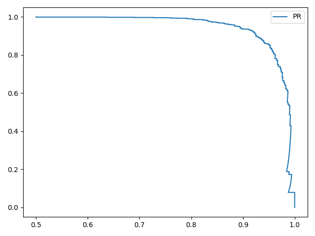
测试2 1 train_images , train_labels, test_images, test_labels = get_two_cate(ratio=1 .0 / 6 )
训练结果如下:
1 2 3 4 5 0.871 # 阈值为0 .5 0.33526167648147953 0.9215 # 阈值为0 .3353
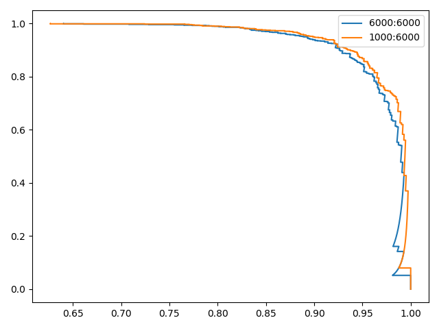
从结果可知,PR曲线同样能够在类别数目不平衡的情况下有效的评估分类器性能
相关阅读 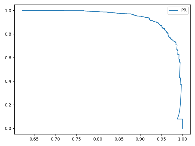
来做第一个留言的人吧!