线性SVM分类器

发表于 2019-07-14 更新于 2021-07-09 分类于机器学习/machine learning 阅读次数：

本文字数： 9.1k 阅读时长 ≈ 17 分钟

最近重温cs231n课程，完成了课堂作业assignment1，记录一下线性SVM分类器相关的概念以及实现

什么是SVM分类器

SVM（support vector machine，支持向量机）分类器定义为特征空间上间隔最大的线性分类器模型，其学习策略是使得分类间隔最大化

线性SVM分类器实现

cs231n上的线性SVM分类器并没有给出数学推导过程，不过其介绍方式更容易理解

SVM分类器训练结果是使得正确类别的成绩至少比错误类别成绩高一个间隔$$

训练过程如下：

首先对输入数据进行线性映射，得到分类成绩；
然后，使用折页损失（hinge loss）函数计算损失值
最后根据损失值进行梯度求导，反向传播

损失值计算

完整的损失值包括折页损失+正则化项

\[ L = \frac {1}{N} \sum_{i} L_{i} + \lambda R(W) \]

折页损失（hinge loss）计算表达式如下：

\[ L_{i} = \sum_{j\neq y_{i}} \max(0, s_{j} - s_{y_{i}} + \triangle ) \]

其中$i$表示批量数据中第$i$个样本，$y_{i}$表示第$i$个样本的正确类别，$j$表示不正确类别

正则化项使用L2范数:

\[ R(W) = \sum_{k} \sum_{l} W_{k,l}^{2} \]

矩阵推导

输入参数：

\[ X \in R^{N\times D} \]

\[ y \in R^{N} \]

\[ W \in R^{D\times C} \]

\[ b \in R^{1\times C} \]

\[ delta \in R^{1} \]

前向计算如下：

\[ scores = X\cdot W + b \in R^{N\times C} \]

\[ corrects = scores[y] \in R^{N\times 1} \]

\[ margins = \frac {1}{N}\sum_{i=1}^{N}\max (0, scores_{i} - corrects_{i} + delta) \]

\[ loss = margins + \lambda R(W) \]

scores = X_batch.dot(self.W) + self.b
correct_class_scores = np.atleast_2d(scores[range(num_train), y_batch]).T
margins = scores - correct_class_scores + delta

loss += np.sum(np.maximum(0, margins)) / num_train
loss += reg * np.sum(self.W ** 2)

反向求导如下：

\[ dmargins = \left\{\begin{matrix} dscores_{i} - dcorrects_{i} & scores_{i} - corrects_{i} + delta > 0\\ 0 & scores_{i} - corrects_{i} + delta <= 0 \end{matrix}\right. \]

dscores = np.zeros(scores.shape)
dscores[margins > 0] = 1
dscores[range(num_train), y_batch] = -1 * np.sum(dscores, axis=1)
dscores /= num_train

权重更新

\[ dW = X^{T} \cdot dscores + reg \cdot W \]

\[ db = \sum_{i=1}^{N}dscores_{i} \]

1 2	dW = X_batch.T.dot(dscores) + reg * self.W db = np.sum(dscores, axis=0)

SVM分类器实现

设置超参数$\triangle =1$

# -*- coding: utf-8 -*-

# @Time    : 19-7-14 下午2:45
# @Author  : zj

import numpy as np


class LinearSVM(object):

    def __init__(self):
        self.W = None
        self.b = None

    def train(self, X, y, learning_rate=1e-3, reg=1e-5, num_iters=100, batch_size=200, verbose=False):
        """
        Inputs:
        - X: A numpy array of shape (N, D) containing training data; there are N
          training samples each of dimension D.
        - y: A numpy array of shape (N,) containing training labels; y[i] = c
          means that X[i] has label 0 <= c < C for C classes.
        - learning_rate: (float) learning rate for optimization.
        - reg: (float) regularization strength.
        - num_iters: (integer) number of steps to take when optimizing
        - batch_size: (integer) number of training examples to use at each step.
        - verbose: (boolean) If true, print progress during optimization.

        Outputs:
        A list containing the value of the loss function at each training iteration.
        """
        num_train, dim = X.shape
        num_classes = np.max(y) + 1  # assume y takes values 0...K-1 where K is number of classes
        if self.W is None:
            # lazily initialize W
            self.W = 0.001 * np.random.randn(dim, num_classes)
            self.b = np.zeros((1, num_classes))

        # Run stochastic gradient descent to optimize W
        loss_history = []
        for it in range(num_iters):
            indices = np.random.choice(num_train, batch_size)
            X_batch = X[indices]
            y_batch = y[indices]

            # evaluate loss and gradient
            loss, dW, db = self.loss(X_batch, y_batch, reg)
            loss_history.append(loss)

            self.W -= learning_rate * dW
            self.b -= learning_rate * db

            if verbose and it % 100 == 0:
                print('iteration %d / %d: loss %f' % (it, num_iters, loss))

        return loss_history

    def predict(self, X):
        """
        Use the trained weights of this linear classifier to predict labels for
        data points.

        Inputs:
        - X: A numpy array of shape (N, D) containing training data; there are N
          training samples each of dimension D.

        Returns:
        - y_pred: Predicted labels for the data in X. y_pred is a 1-dimensional
          array of length N, and each element is an integer giving the predicted
          class.
        """
        scores = X.dot(self.W)
        y_pred = np.argmax(scores, axis=1)

        return y_pred

    def loss(self, X_batch, y_batch, reg, delta=1):
        """
        Compute the loss function and its derivative.
        Subclasses will override this.

        Inputs:
        - X_batch: A numpy array of shape (N, D) containing a minibatch of N
          data points; each point has dimension D.
        - y_batch: A numpy array of shape (N,) containing labels for the minibatch.
        - reg: (float) regularization strength.

        Returns: A tuple containing:
        - loss as a single float
        - gradient with respect to self.W; an array of the same shape as W
        """
        loss = 0.0
        num_train = X_batch.shape[0]

        scores = X_batch.dot(self.W) + self.b
        correct_class_scores = np.atleast_2d(scores[range(num_train), y_batch]).T
        margins = scores - correct_class_scores + delta

        loss += np.sum(np.maximum(0, margins)) / num_train
        loss += reg * np.sum(self.W ** 2)

        dscores = np.zeros(scores.shape)
        dscores[margins > 0] = 1
        dscores[range(num_train), y_batch] = -1 * np.sum(dscores, axis=1)
        dscores /= num_train

        dW = X_batch.T.dot(dscores) + reg * self.W
        db = np.sum(dscores, axis=0)

        return loss, dW, db

实验

针对Iris数据集和German data数据集进行SVM分类器训练，完整代码如下：

# -*- coding: utf-8 -*-

# @Time    : 19-7-15 下午1:50
# @Author  : zj


from builtins import range
from classifier.svm_classifier import LinearSVM
import pandas as pd
import numpy as np
import math
from sklearn import utils
from sklearn.model_selection import train_test_split
import matplotlib.pyplot as plt
import warnings

warnings.filterwarnings("ignore")


def load_iris(iris_path, shuffle=True, tsize=0.8):
    """
    加载iris数据
    """
    data = pd.read_csv(iris_path, header=0, delimiter=',')

    if shuffle:
        data = utils.shuffle(data)

    species_dict = {
        'Iris-setosa': 0,
        'Iris-versicolor': 1,
        'Iris-virginica': 2
    }
    data['Species'] = data['Species'].map(species_dict)

    data_x = np.array(
        [data['SepalLengthCm'], data['SepalWidthCm'], data['PetalLengthCm'], data['PetalWidthCm']]).T
    data_y = data['Species']

    x_train, x_test, y_train, y_test = train_test_split(data_x, data_y, train_size=tsize, test_size=(1 - tsize),
                                                        shuffle=False)

    return np.array(x_train), np.array(x_test), np.array(y_train), np.array(y_test)


def load_german_data(data_path, shuffle=True, tsize=0.8):
    data_list = pd.read_csv(data_path, header=None, sep='\s+')

    data_array = data_list.values
    height, width = data_array.shape[:2]
    data_x = data_array[:, :(width - 1)]
    data_y = data_array[:, (width - 1)]

    x_train, x_test, y_train, y_test = train_test_split(data_x, data_y, train_size=tsize, test_size=(1 - tsize),
                                                        shuffle=shuffle)

    y_train = np.array(list(map(lambda x: 1 if x == 2 else 0, y_train)))
    y_test = np.array(list(map(lambda x: 1 if x == 2 else 0, y_test)))

    return x_train, x_test, y_train, y_test


def compute_accuracy(y, y_pred):
    num = y.shape[0]
    num_correct = np.sum(y_pred == y)
    acc = float(num_correct) / num
    return acc


def cross_validation(x_train, y_train, x_val, y_val, lr_choices, reg_choices):
    results = {}
    best_val = -1  # The highest validation accuracy that we have seen so far.
    best_svm = None  # The LinearSVM object that achieved the highest validation rate.

    for lr in lr_choices:
        for reg in reg_choices:
            svm = LinearSVM()

            svm.train(x_train, y_train, learning_rate=lr, reg=reg, num_iters=2000, batch_size=100, verbose=True)
            y_train_pred = svm.predict(x_train)
            y_val_pred = svm.predict(x_val)

            train_acc = np.mean(y_train_pred == y_train)
            val_acc = np.mean(y_val_pred == y_val)

            results[(lr, reg)] = (train_acc, val_acc)
            if best_val < val_acc:
                best_val = val_acc
                best_svm = svm

    return results, best_svm, best_val


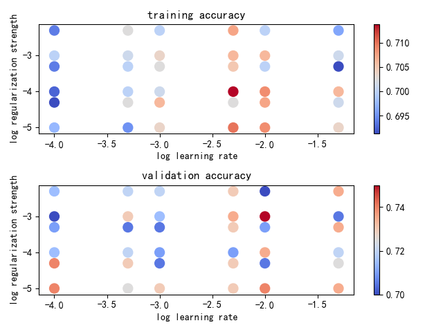
def plot(results):
    # Visualize the cross-validation results
    x_scatter = [math.log10(x[0]) for x in results]
    y_scatter = [math.log10(x[1]) for x in results]

    # plot training accuracy
    marker_size = 100
    colors = [results[x][0] for x in results]
    plt.subplot(2, 1, 1)
    plt.scatter(x_scatter, y_scatter, marker_size, c=colors, cmap=plt.cm.coolwarm)
    plt.colorbar()
    plt.xlabel('log learning rate')
    plt.ylabel('log regularization strength')
    plt.title('training accuracy')

    # plot validation accuracy
    colors = [results[x][1] for x in results]  # default size of markers is 20
    plt.subplot(2, 1, 2)
    plt.scatter(x_scatter, y_scatter, marker_size, c=colors, cmap=plt.cm.coolwarm)
    plt.colorbar()
    plt.xlabel('log learning rate')
    plt.ylabel('log regularization strength')
    plt.title('validation accuracy')
    plt.show()


if __name__ == '__main__':
    iris_path = '/home/zj/data/iris-species/Iris.csv'
    x_train, x_test, y_train, y_test = load_iris(iris_path, shuffle=True, tsize=0.8)

    # data_path = '/home/zj/data/german/german.data-numeric'
    # x_train, x_test, y_train, y_test = load_german_data(data_path, shuffle=True, tsize=0.8)

    x_train = x_train.astype(np.double)
    x_test = x_test.astype(np.double)
    mu = np.mean(x_train, axis=0)
    var = np.var(x_train, axis=0)
    eps = 1e-8
    x_train = (x_train - mu) / np.sqrt(var + eps)
    x_test = (x_test - mu) / np.sqrt(var + eps)

    lr_choices = [1e-4, 5e-4, 1e-3, 5e-3, 1e-2, 5e-2]
    reg_choices = [1e-4, 5e-4, 1e-3, 5e-3, 1e-2, 5e-2]
    results, best_svm, best_val = cross_validation(x_train, y_train, x_test, y_test, lr_choices, reg_choices)

    plot(results)

    for k in results.keys():
        lr, reg = k
        train_acc, val_acc = results[k]
        print('lr = %f, reg = %f, train_acc = %f, val_acc = %f' % (lr, reg, train_acc, val_acc))

    print('最好的设置是： lr = %f, reg = %f' % (best_svm.lr, best_svm.reg))
    print('最好的测试精度： %f' % best_val)

测试不同学习率和正则化强度下的SVM分类器训练结果，批量大小为100，每组参数训练2000次

Iris数据集训练结果如下：

1 2	最好的设置是： lr = 0.001000, reg = 0.000100 最好的测试精度： 0.800000

German data数据集训练结果如下：

1 2	最好的设置是： lr = 0.010000, reg = 0.001000 最好的测试精度： 0.750000

小结

	Iris	German data
KNN	93.33%	73.5%
SVM	80%	75%

线性SVM分类器对于非线性数据的分类结果不理想。不过可以通过核技巧，将原始特征投影到高维空间，从而能够实现非线性SVM分类器，进一步提高分类性能

大海