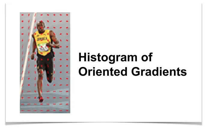
[译]Histogram of Oriented Gradients
方向梯度直方图(Histogram Of Oriented Gradients,简称为HOG)是常用的纹理特征之一,本篇文章简单易懂的讲解了HOG概念
原文地址:Histogram of Oriented Gradients
In this post, we will learn the details of the Histogram of Oriented Gradients (HOG) feature descriptor. We will learn what is under the hood and how this descriptor is calculated internally by OpenCV, MATLAB and other packages.
在这篇文章中,我们将学习方向梯度直方图(HOG)特征描述的细节。我们将学习概念背后的内容,以及如何通过OpenCV、MATLAB和其他软件包在内部计算这个描述符
This post is part of a series I am writing on Image Recognition and Object Detection.
这篇文章是我正在写的关于图像识别和目标检测的系列文章的一部分
The complete list of tutorials in this series is given below:
Image recognition using traditional Computer Vision techniques : Part 1
Histogram of Oriented Gradients : Part 2
Example code for image recognition : Part 3
Training a better eye detector: Part 4a
Object detection using traditional Computer Vision techniques : Part 4b
How to train and test your own OpenCV object detector : Part 5
Image recognition using Deep Learning : Part 6
- Introduction to Neural Networks
- Understanding Feedforward Neural Networks
- Image Recognition using Convolutional Neural Networks
Object detection using Deep Learning : Part 7
本系列教程的完整列表如下:
- 使用传统计算机视觉技术的图像识别:Part 1
- 方向梯度直方图:Part 2
- 图像识别示例代码:Part 3
- 训练一个更好的眼睛探测器:Part 4a
- 基于传统计算机视觉技术的目标检测:Part 4b
- 如何训练和测试自己的OpenCV对象检测器:Part 5
- 基于深度学习的图像识别:Part 6
- 神经网络介绍
- 理解前向神经网络
- 使用卷积神经网络进行图像识别
- 使用深度学习的目标识别:Part 7
A lot many things look difficult and mysterious. But once you take the time to deconstruct them, the mystery is replaced by mastery and that is what we are after. If you are a beginner and are finding Computer Vision hard and mysterious, just remember the following
Q : How do you eat an elephant ? A : One bite at a time!
很多事情看起来既困难又神秘。但一旦你花时间去解构它们,神秘就被掌握所取代,这就是我们所追求的。如果你是一个初学者,发现计算机视觉很难而且很神秘,请记住以下几点
问题:如何吃掉一头大象?
答案:一口一口的吃!
What is a Feature Descriptor
什么是特征描述符
A feature descriptor is a representation of an image or an image patch that simplifies the image by extracting useful information and throwing away extraneous information.
特征描述符是通过提取有用信息和丢弃无关信息来简化图像的图像或图像块的表示
Typically, a feature descriptor converts an image of size width x height x 3 (channels ) to a feature vector / array of length n. In the case of the HOG feature descriptor, the input image is of size 64 x 128 x 3 and the output feature vector is of length 3780.
通常,特征描述符将大小为宽x高x3(通道数)的图像转换为长度为n的特征向量/阵列。在HOG特征描述符的情况下,输入图像的大小为64x128x3,输出特征向量的长度为3780
Keep in mind that HOG descriptor can be calculated for other sizes, but in this post I am sticking to numbers presented in the original paper so you can easily understand the concept with one concrete example.
请记住,HOG描述符可以计算其他大小,但在本文中,我将坚持在原始论文中给出的数字,这样您就可以通过一个具体的例子轻松理解这个概念
This all sounds good, but what is "useful" and what is "extraneous"? To define "useful", we need to know what is it "useful" for? Clearly, the feature vector is not useful for the purpose of viewing the image. But, it is very useful for tasks like image recognition and object detection. The feature vector produced by these algorithms when fed into an image classification algorithms like Support Vector Machine (SVM) produce good results.
这听起来不错,但什么是“有用的”和什么是“无关的”?要定义“有用”,我们需要知道它“有用”目的是什么?显然,特征向量对于查看图像是没有用处的。但是,它对于图像识别和目标检测等任务非常有用。将这些算法产生的特征向量输入到支持向量机(SVM)等图像分类算法中,可以得到较好的分类效果
But, what kinds of "features" are useful for classification tasks? Let’s discuss this point using an example. Suppose we want to build an object detector that detects buttons of shirts and coats. A button is circular ( may look elliptical in an image ) and usually has a few holes for sewing. You can run an edge detector on the image of a button, and easily tell if it is a button by simply looking at the edge image alone. In this case, edge information is "useful" and color information is not. In addition, the features also need to have discriminative power. For example, good features extracted from an image should be able to tell the difference between buttons and other circular objects like coins and car tires.
但是,什么样的“特征”对分类任务有用呢?让我们用一个例子来讨论这一点。假设我们想建立一个目标探测器来检测衬衫和外套的纽扣。按钮是圆形的(在图像中可能看起来是椭圆形的),通常有几个缝孔。你可以在按钮的图像上运行一个边缘检测器,只需简单地查看边缘图像就可以很容易地判断它是否是按钮。在这种情况下,边缘信息是“有用的”,而颜色信息则不是。此外,这些特征还需要有辨别力。例如,从图像中提取的良好特征应该能够区分按钮和其他圆形物体(如硬币和汽车轮胎)之间的区别
In the HOG feature descriptor, the distribution (histograms) of directions of gradients (oriented gradients) are used as features. Gradients (x and y derivatives) of an image are useful because the magnitude of gradients is large around edges and corners (regions of abrupt intensity changes) and we know that edges and corners pack in a lot more information about object shape than flat regions.
在HOG特征描述符中,使用梯度方向(定向梯度)的分布(直方图)作为特征。图像的梯度(x和y导数)是有用的,因为边缘和角落(强度突变区域)的梯度幅度很大,我们知道边缘和角落比平面区域包含更多关于目标形状的信息
How to calculate Histogram of Oriented Gradients ?
如何计算方向导数直方图?
In this section, we will go into the details of calculating the HOG feature descriptor. To illustrate each step, we will use a patch of an image.
在本节中,我们将详细讨论计算HOG特征描述符。为了说明每个步骤,我们将使用一个图像块
Step 1: Preprocessing
第一步:预处理
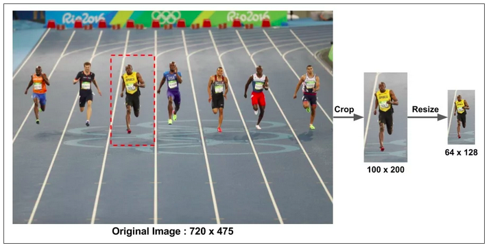
As mentioned earlier HOG feature descriptor used for pedestrian detection is calculated on a 64×128 patch of an image. Of course, an image may be of any size. Typically patches at multiple scales are analyzed at many image locations. The only constraint is that the patches being analyzed have a fixed aspect ratio. In our case, the patches need to have an aspect ratio of 1:2. For example, they can be 100×200, 128×256, or 1000×2000 but not 101×205.
如前所述,用于行人检测的HOG特征描述符是在图像的64×128大小的块上计算的。当然,图像可以是任何大小。通常在多个图像位置分析多个尺度的图像块。唯一的限制是所分析的图像块具有固定的长宽比。在我们的例子中,补丁需要有1:2的长宽比。例如,它们可以是100×200、128×256或1000×2000,但不能是101×205
To illustrate this point I have shown a large image of size 720×475. We have selected a patch of size 100×200 for calculating our HOG feature descriptor. This patch is cropped out of an image and resized to 64×128. Now we are ready to calculate the HOG descriptor for this image patch.
为了说明这一点,我展示了一幅720×475的大图像。我们选择了一个大小为100×200的块来计算我们的HOG特征描述符。此图像块将从图像中裁剪并调整大小为64×128。现在我们可以计算这个图像块的HOG描述符了
The paper by Dalal and Triggs also mentions gamma correction as a preprocessing step, but the performance gains are minor and so we are skipping the step.
Dalal和Triggs的论文也提到gamma校正是一个预处理步骤,但是性能提高很小,所以我们跳过了这个步骤
Step 2: Calculate the Gradient Images
第二步:计算梯度图像
To calculate a HOG descriptor, we need to first calculate the horizontal and vertical gradients; after all, we want to calculate the histogram of gradients. This is easily achieved by filtering the image with the following kernels.
要计算HOG描述符,首先需要计算水平和垂直梯度;毕竟,我们要计算梯度的直方图。这很容易通过使用以下内核过滤图像来实现
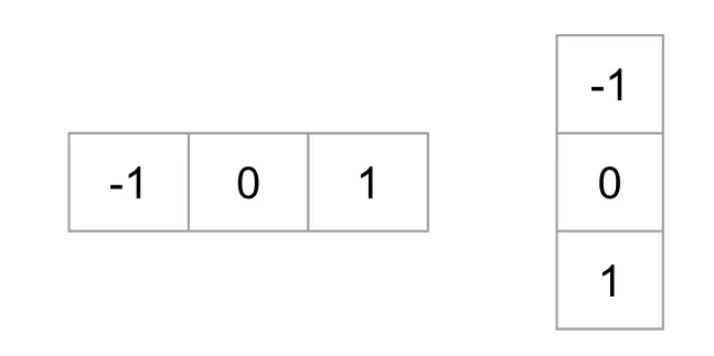
We can also achieve the same results, by using Sobel operator in OpenCV with kernel size 1.
在OpenCV中使用核大小为1的Sobel算子也可以得到同样的结果
1 | // C++ gradient calculation. |
Next, we can find the magnitude and direction of gradient using the following formula
下一步,我们可以用下面的公式找到梯度的大小和方向
\[ g=\sqrt{g_{x}^{2} + g_{y}^{2}} \\ \theta = \arctan \frac{g_{y}}{g_{x}} \]
If you are using OpenCV, the calculation can be done using the function cartToPolar as shown below.
如果使用OpenCV,可以使用函数cartToPolar完成计算,如下所示
1 | // C++ Calculate gradient magnitude and direction (in degrees) |
The figure below shows the gradients.
下图显示了梯度结果
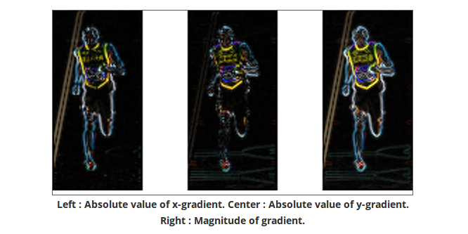
Left : Absolute value of x-gradient. Center : Absolute value of y-gradient. Right : Magnitude of gradient.
左图:x轴方向梯度大小;中间:y轴方向梯度大小;右图:x-y轴梯度大小
Notice, the x-gradient fires on vertical lines and the y-gradient fires on horizontal lines. The magnitude of gradient fires where ever there is a sharp change in intensity. None of them fire when the region is smooth. I have deliberately left out the image showing the direction of gradient because direction shown as an image does not convey much.
注意,x轴梯度在垂直线上激发,y轴梯度在水平线上激发。梯度在像素强度剧烈变化的地方激发。当区域平滑时,它们都不会被激发。我故意忽略了显示梯度方向的图像,因为显示图像的方向传达不了太多信息
The gradient image removed a lot of non-essential information ( e.g. constant colored background ), but highlighted outlines. In other words, you can look at the gradient image and still easily say there is a person in the picture.
梯度图像去除了很多不必要的信息(如恒定的彩色背景),但突出了轮廓。换言之,看到梯度图像仍然可以很容易地发现有一个人在图片中
At every pixel, the gradient has a magnitude and a direction. For color images, the gradients of the three channels are evaluated ( as shown in the figure above ). The magnitude of gradient at a pixel is the maximum of the magnitude of gradients of the three channels, and the angle is the angle corresponding to the maximum gradient.
在每个像素处,梯度都有大小和方向。对于彩色图像,需要各自计算三个通道的梯度(如上图所示)。在一个像素处的梯度幅度是三个通道梯度的最大值,并且角度是对应于最大梯度的角度
Step 3: Calculate Histogram of Gradients in 8x8 cells
第三步:计算8x8个单元格中的梯度直方图
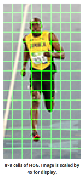
In this step, the image is divided into 8×8 cells and a histogram of gradients is calculated for each 8×8 cells.
在这一步中,图像被分成8×8大小的单元格,并为每个8×8大小单元格计算梯度直方图
We will learn about the histograms in a moment, but before we go there let us first understand why we have divided the image into 8×8 cells. One of the important reasons to use a feature descriptor to describe a patch of an image is that it provides a compact representation. An 8×8 image patch contains 8x8x3 = 192 pixel values. The gradient of this patch contains 2 values ( magnitude and direction ) per pixel which adds up to 8x8x2 = 128 numbers. By the end of this section we will see how these 128 numbers are represented using a 9-bin histogram which can be stored as an array of 9 numbers. Not only is the representation more compact, calculating a histogram over a patch makes this represenation more robust to noise. Individual graidents may have noise, but a histogram over 8×8 patch makes the representation much less sensitive to noise.
我们稍后将学习直方图,但在我们开始学习之前,让我们先了解一下为什么我们将图像划分到8×8大小单元格。使用特征描述符描述图像的一个重要原因是它提供了一个紧凑的表示。8×8图像块包含8x8x3=192像素值。此图像块的梯度包含每个像素2个值(大小和方向),总计为8x8x2=128个数字。在本节结束时,我们将看到如何使用一个9-bin大小直方图来表示这128个数字,该直方图可以存储为一个由9个数字组成的数组。不仅表示更紧凑,计算一个补丁上的直方图使这种表示对噪声更具有鲁棒性。单个梯度可能有噪声,但是8×8大小图象块的直方图使表示对噪声的敏感性大大降低
But why 8×8 patch ? Why not 32×32 ? It is a design choice informed by the scale of features we are looking for. HOG was used for pedestrian detection initially. 8×8 cells in a photo of a pedestrian scaled to 64×128 are big enough to capture interesting features ( e.g. the face, the top of the head etc. ).
但是为什么是8×8补丁呢?为什么不是32×32?这是一个设计选择,由我们正在寻找的功能的规模所决定。HOG最初用于行人检测。一张行人照片中的8×8格放大到64×128,足以捕捉有趣的特征(如面部、头顶等)
The histogram is essentially a vector ( or an array ) of 9 bins ( numbers ) corresponding to angles 0, 20, 40, 60 … 160.
直方图本质上是一个由9个格(数字)组成的向量(或数组),对应于0、20、40、60…160的角度
Let us look at one 8×8 patch in the image and see how the gradients look.
让我们来看看图像中的一个8×8大小的补丁,看看梯度是什么样子的
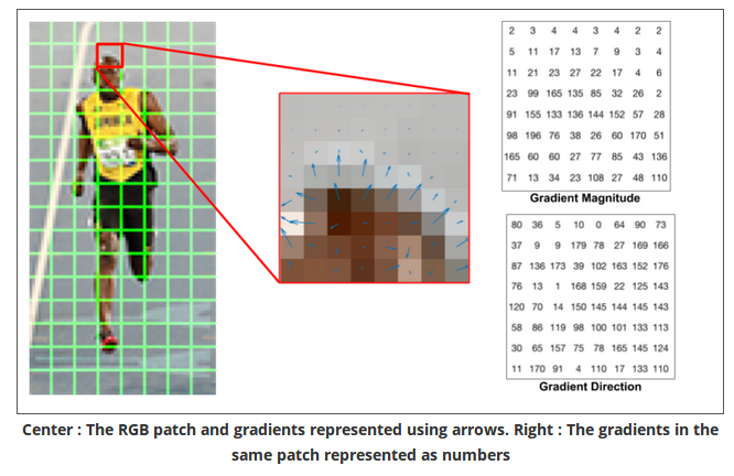
Center : The RGB patch and gradients represented using arrows. Right : The gradients in the same patch represented as numbers
左图:RGB块以及箭头表示的梯度;右图:用数值表示图像块各个像素的梯度大小和方向
If you are a beginner in computer vision, the image in the center is very informative. It shows the patch of the image overlaid with arrows showing the gradient — the arrow shows the direction of gradient and its length shows the magnitude. Notice how the direction of arrows points to the direction of change in intensity and the magnitude shows how big the difference is.
如果你是计算机视觉的初学者,左图的信息量很大。它表示图像块,上面覆盖着表示梯度的箭头 - 箭头表示梯度的方向,其长度表示大小。请注意箭头方向指向强度变化的方向,而大小显示了差异有多大
On the right, we see the raw numbers representing the gradients in the 8×8 cells with one minor difference — the angles are between 0 and 180 degrees instead of 0 to 360 degrees. These are called “unsigned” gradients because a gradient and it’s negative are represented by the same numbers. In other words, a gradient arrow and the one 180 degrees opposite to it are considered the same. But, why not use the 0 – 360 degrees ? Empirically it has been shown that unsigned gradients work better than signed gradients for pedestrian detection. Some implementations of HOG will allow you to specify if you want to use signed gradients.
右图中,我们看到代表8×8单元格中梯度的原始数字,只有一个微小的差异-角度在0到180度之间,而不是0到360度之间。这些称为“无符号”梯度,因为梯度和它的负数由相同的数字表示。换句话说,梯度箭头和与之相对的180度箭头被认为是相同的。但是,为什么不使用0-360度呢?经验表明,无符号梯度比有符号梯度更适合行人检测。HOG的一些实现允许您指定是否要使用带符号的渐变
The next step is to create a histogram of gradients in these 8×8 cells. The histogram contains 9 bins corresponding to angles 0, 20, 40 … 160.
下一步是在这些8×8单元格中创建梯度直方图。直方图包含9个对应于角度0、20、40…160的区域
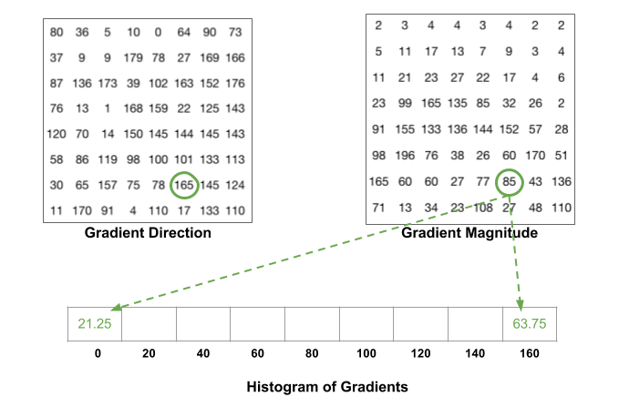
The following figure illustrates the process. We are looking at magnitude and direction of the gradient of the same 8×8 patch as in the previous figure. A bin is selected based on the direction, and the vote ( the value that goes into the bin ) is selected based on the magnitude. Let’s first focus on the pixel encircled in blue. It has an angle ( direction ) of 80 degrees and magnitude of 2. So it adds 2 to the 5th bin. The gradient at the pixel encircled using red has an angle of 10 degrees and magnitude of 4. Since 10 degrees is half way between 0 and 20, the vote by the pixel splits evenly into the two bins.
下图说明了该过程。我们正在研究同一个8×8图像块的梯度大小和方向,如上图所示。根据方向选择一个bin,并根据大小选择投票(进入bin的值)。让我们首先关注蓝色圈出的像素。它的角度(方向)为80度,大小为2,所以第五个bin加2。使用红色圈出的像素的梯度角度为10度,大小为4。由于10度是0到20之间的一半,因此按像素进行的投票将均匀地分成两个容器
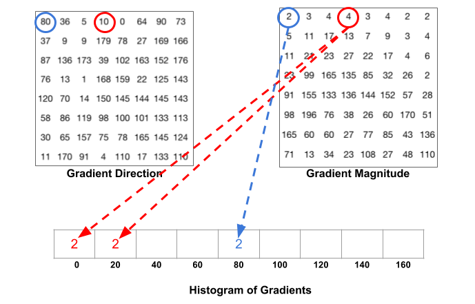
There is one more detail to be aware of. If the angle is greater than 160 degrees, it is between 160 and 180, and we know the angle wraps around making 0 and 180 equivalent. So in the example below, the pixel with angle 165 degrees contributes proportionally to the 0 degree bin and the 160 degree bin.
还有一个细节需要注意。如果角度大于160度,它在160到180之间,我们知道角度在0到180之间。因此在下面的例子中,角度为165度的像素值成比例的分配给0度和160度的bin
The contributions of all the pixels in the 8×8 cells are added up to create the 9-bin histogram. For the patch above, it looks like this
将8×8单元格中所有像素按分布相加,生成9-bin直方图。上面的图像块得到如下结果
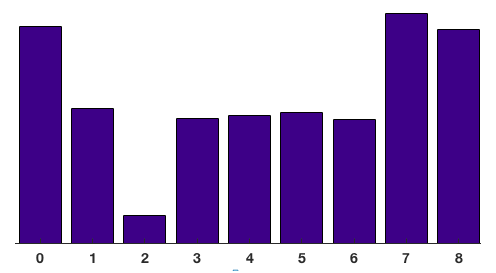
In our representation, the y-axis is 0 degrees. You can see the histogram has a lot of weight near 0 and 180 degrees, which is just another way of saying that in the patch gradients are pointing either up or down.
在我们的表示中,y轴是0度。你可以看到直方图在0度和180度附近有很多权重值,换一种说法就是在图像块中梯度要么指向上,要么指向下
Step 4: 16x16 Block Normalization
第四步:16x16大小的块标准化
In the previous step, we created a histogram based on the gradient of the image. Gradients of an image are sensitive to overall lighting. If you make the image darker by dividing all pixel values by 2, the gradient magnitude will change by half, and therefore the histogram values will change by half. Ideally, we want our descriptor to be independent of lighting variations. In other words, we would like to "normalize" the histogram so they are not affected by lighting variations.
上一步中计算了图像的梯度直方图。图像的梯度对整体照明敏感。如果将所有像素值除以2使图像变暗,则梯度大小将更改一半,因此直方图值将更改一半。理想情况下,我们希望描述符独立于光照变化。换言之,我们希望"标准化"直方图,使其不受光照变化的影响
Before I explain how the histogram is normalized, let’s see how a vector of length 3 is normalized.
在解释直方图是如何标准化之前,让我们看看长度为3的向量是如何标准化的
Let’s say we have an RGB color vector [ 128, 64, 32 ]. The length of this vector is \(\sqrt{128^2 + 64^2 + 32^2} = 146.64\). This is also called the L2 norm of the vector. Dividing each element of this vector by 146.64 gives us a normalized vector [0.87, 0.43, 0.22]. Now consider another vector in which the elements are twice the value of the first vector 2 x [ 128, 64, 32 ] = [ 256, 128, 64 ]. You can work it out yourself to see that normalizing [ 256, 128, 64 ] will result in [0.87, 0.43, 0.22], which is the same as the normalized version of the original RGB vector. You can see that normalizing a vector removes the scale.
假设我们有一个RGB颜色向量[128,64,32]。向量长度是\(\sqrt{128^2 + 64^2 + 32^2} = 146.64\)。这也被称为向量的L2范数。将这个向量的每个元素除以146.64,得到一个标准化向量[0.87,0.43,0.22]。现在考虑另一个向量,其中的元素是第一个向量的两倍:2x[128,64,32]=[256,128,64]。通过计算可知标准化[256,128,64]将得到[0.87,0.43,0.22],这与原始RGB向量的标准化结果相同。所以标准化操作移除了尺度的影响
Now that we know how to normalize a vector, you may be tempted to think that while calculating HOG you can simply normalize the 9×1 histogram the same way we normalized the 3×1 vector above. It is not a bad idea, but a better idea is to normalize over a bigger sized block of 16×16. A 16×16 block has 4 histograms which can be concatenated to form a 36 x 1 element vector and it can be normalized just the way a 3×1 vector is normalized. The window is then moved by 8 pixels ( see animation ) and a normalized 36×1 vector is calculated over this window and the process is repeated.
现在我们知道了如何标准化向量,您可能会想,在计算HOG时,您可以简单地规范化9×1直方图,就像我们规范化上面的3×1向量一样。这不是个坏主意,但更好的办法是在更大的16×16的块上进行标准化。一个16x16大小的块有四个直方图,这些直方图可以连接起来形成一个36x1大小的向量,并且按照这种方式进行标准化。每次标准化将窗口移动8个像素(参见动画),并在此窗口上计算标准化的36×1矢量,然后重复该过程
Step 5: Calculate the HOG feature vector
第5步:计算HOG特征向量
To calculate the final feature vector for the entire image patch, the 36×1 vectors are concatenated into one giant vector. What is the size of this vector ? Let us calculate
为了计算整个图像块的最终特征向量,将36×1的向量拼接成一个巨大的向量。这个向量的大小是多少?让我们计算一下
- How many positions of the 16×16 blocks do we have ? There are 7 horizontal and 15 vertical positions making a total of 7 x 15 = 105 positions.
- Each 16×16 block is represented by a 36×1 vector. So when we concatenate them all into one gaint vector we obtain a 36×105 = 3780 dimensional vector.
- 我们16×16大小的图像块有多少个位置?共有7个水平位置和15个垂直位置(输入图像大小为64x128),共计7x15=105个位置
- 每个16×16块代表36×1向量,连接在一起得到了一个36×105=3780维大小的向量
Visualizing Histogram of Oriented Gradients
可视化方向梯度直方图
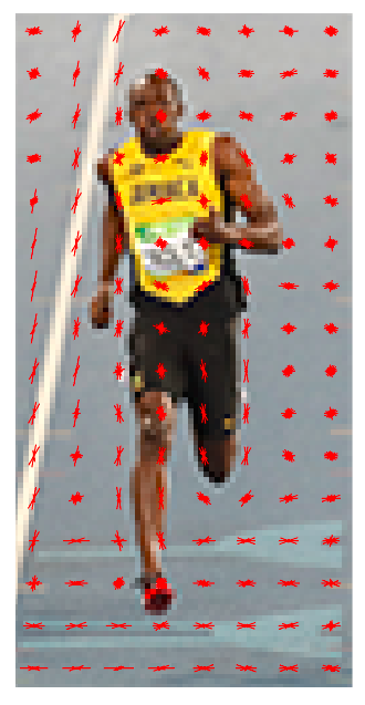
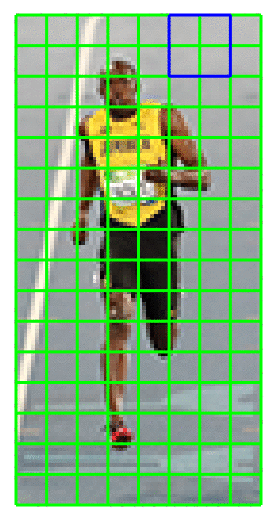
The HOG descriptor of an image patch is usually visualized by plotting the 9×1 normalized histograms in the 8×8 cells. See image on the side. You will notice that dominant direction of the histogram captures the shape of the person, especially around the torso and legs.
图像块的HOG描述符通常是通过在8×8单元格中绘制9×1的归一化直方图来实现的。参考下面图片。你会注意到直方图的主导方向捕捉到了人的形状,尤其是躯干和腿部
Unfortunately, there is no easy way to visualize the HOG descriptor in OpenCV.
不幸的是,在OpenCV中没有简单的方法可以可视化HOG描述符