[译]高效的基于图的图像分割
论文及C++实现下载地址:Efficient Graph-Based Image Segmentation
摘要
This paper addresses the problem of segmenting an image into regions. We define a predicate for measuring the evidence for a boundary between two regions using a graph-based representation of the image. We then develop an efficient segmentation algorithm based on this predicate, and show that although this algorithm makes greedy decisions it produces segmentations that satisfy global properties. We apply the algorithm to image segmentation using two different kinds of local neighborhoods in constructing the graph, and illustrate the results with both real and synthetic images. The algorithm runs in time nearly linear in the number of graph edges and is also fast in practice. An important characteristic of the method is its ability to preserve detail in low-variability image regions while ignoring detail in high-variability regions.
本文讨论了将图像分割成区域的问题。我们定义了一个谓词,用于使用基于图的图像表示来测量两个区域之间边界的证据。然后,我们开发了一种基于该谓词的高效分割算法,并证明了尽管该算法做出贪婪决策,但它产生满足全局属性的分割。将该算法应用于图像分割中,利用两种不同的局部邻域构造图像,并用真实图像和合成图像对结果进行了说明。算法运行时间与图像边缘数呈线性关系,而且在实际应用中也很快。该方法的一个重要特点是在低变率图像区域(低频区域)保留细节,而在高变率区域(高频区域)忽略细节
引言
The problems of image segmentation and grouping remain great challenges for computer vision. Since the time of the Gestalt movement in psychology (e.g., [17]), it has been known that perceptual grouping plays a powerful role in human visual perception. A wide range of computational vision problems could in principle make good use of segmented images, were such segmentations reliably and efficiently computable. For instance intermediate-level vision problems such as stereo and motion estimation require an appropriate region of support for correspondence operations. Spatially non-uniform regions of support can be identified using segmentation techniques. Higher-level problems such as recognition and image indexing can also make use of segmentation results in matching, to address problems such as figure-ground separation and recognition by parts.
图像分割和分组问题一直是计算机视觉面临的巨大挑战。从心理学的格式塔运动(如[17])开始,人们就知道知觉组织在人类视觉感知中起着重要作用。如果这种分割是可靠和有效的计算,那么原则上可以在广泛的计算视觉问题中很好地利用分割图像。例如,中级视觉问题,如立体和运动估计,需要一个适当的区域来支持对应操作。空间上不均匀的支持区域可以用分割技术来识别。更高层次的问题,如识别和图像索引,也可以利用分割结果进行匹配,以解决图形-背景分离和部分识别等问题
Our goal is to develop computational approaches to image segmentation that are broadly useful, much in the way that other low-level techniques such as edge detection are used in a wide range of computer vision tasks. In order to achieve such broad utility, we believe it is important that a segmentation method have the following properties:
我们的目标是开发出广泛有用的图像分割的计算方法,这与其他低级技术(如边缘检测)在广泛的计算机视觉任务中的使用方式非常相似。为了实现如此广泛的实用性,我们认为分割方法应该具有以下重要特性:
- Capture perceptually important groupings or regions, which often reflect global aspects of the image. Two central issues are to provide precise characterizations of what is perceptually important, and to be able to specify what a given segmentation technique does. We believe that there should be precise definitions of the properties of a resulting segmentation, in order to better understand the method as well as to facilitate the comparison of different approaches.
- Be highly efficient, running in time nearly linear in the number of image pixels. In order to be of practical use, we believe that segmentation methods should run at speeds similar to edge detection or other low-level visual processing techniques, meaning nearly linear time and with low constant factors. For example, a segmentation technique that runs at several frames per second can be used in video processing applications.
捕捉感知上重要的组织或区域,这些组织或区域通常反映图像的全局内容。有两个核心问题,一是提供对感知重要的东西的精确描述,二是能够指定给定的分割技术所做的工作。我们认为,为了更好地理解该方法,并便于比较不同方法,应该对结果分割的属性有精确的定义
高效率运行,即图像像素数与运行时间呈线性关系。为了实际应用,我们认为分割方法应该以类似于边缘检测或其他低级视觉处理技术的速度运行,这意味着几乎是线性时间,具有较低的常数因子。例如,视频处理应用程序中可以使用每秒几帧的分割技术。
While the past few years have seen considerable progress in eigenvector-based methods of image segmentation (e.g., [14, 16]), these methods are too slow to be practical for many applications. In contrast, the method described in this paper has been used in large-scale image database applications as described in [13]. While there are other approaches to image segmentation that are highly efficient, these methods generally fail to capture perceptually important non-local properties of an image as discussed below. The segmentation technique developed here both captures certain perceptually important non-local image characteristics and is computationally efficient – running in O(n log n) time for n image pixels and with low constant factors, and can run in practice at video rates.
虽然在过去的几年里,基于特征向量的图像分割方法(如[14,16])取得了相当大的进展,但这些方法的速度太慢,不适合许多应用。相比之下,本文所述的方法已用于大型图像数据库应用,如[13]所述。虽然有其他方法可以高效地进行图像分割,但这些方法通常无法捕获如下文所述图像中感知重要的非局部特性。本文实现的分割技术不仅捕获了某些重要的感知非局部图像特征,而且计算效率高 - 在O(nlogn)时间内运行n个图像像素,且常数因子较低,可以在实际中以视频速率运行
As with certain classical clustering methods [15, 19], our method is based on selecting edges from a graph, where each pixel corresponds to a node in the graph, and certain neighboring pixels are connected by undirected edges. Weights on each edge measure the dissimilarity between pixels. However, unlike the classical methods, our technique adaptively adjusts the segmentation criterion based on the degree of variability in neighboring regions of the image. This results in a method that, while making greedy decisions, can be shown to obey certain non-obvious global properties. We also show that other adaptive criteria, closely related to the one developed here, result in problems that are computationally difficult (NP hard).
与某些经典的聚类方法[15,19]一样,我们的方法基于从图中选择边,其中每个像素对应于图中的一个节点,并且某些相邻像素由无向边连接。每个边上的权重测量像素之间的差异。但是,与传统方法不同,我们的技术根据图像相邻区域的变化程度自适应调整分割标准。这就产生了一种方法,在做出贪婪决定时,可以证明它服从某些不明显的全局属性。我们还表明,与这里开发的自适应标准密切相关的其他自适应标准会导致计算困难(NP困难)的问题
We now turn to a simple synthetic example illustrating some of the non-local image characteristics captured by our segmentation method. Consider the image shown in the top left of Figure 1. Most people will say that this image has three distinct regions: a rectangular-shaped intensity ramp in the left half, a constant intensity region with a hole on the right half, and a high-variability rectangular region inside the constant region. This example illustrates some perceptually important properties that we believe should be captured by a segmentation algorithm. First, widely varying intensities should not alone be judged as evidence for multiple regions. Such wide variation in intensities occurs both in the ramp on the left and in the high variability region on the right. Thus it is not adequate to assume that regions have nearly constant or slowly varying intensities.
现在我们来看一个简单的合成例子,说明我们的分割方法捕获的一些非局部图像特征。考虑图1左上角所示的图像。大多数人会说,这幅图像有三个不同的区域:左半部分有一个矩形的强度渐变,右半部分有一个孔的恒定强度区域,以及恒定区域内的高变率矩形区域。这个例子说明了一些我们认为应该由分割算法捕获的重要感知属性。首先,广泛变化的强度不应单独作为多个区域的证据。这种强度的巨大变化既发生在左侧的斜坡上,也发生在右侧的高变率区域。因此,不足以假设区域具有几乎恒定或缓慢变化的强度
A second perceptually important aspect of the example in Figure 1 is that the three meaningful regions cannot be obtained using purely local decision criteria. This is because the intensity difference across the boundary between the ramp and the constant region is actually smaller than many of the intensity differences within the high variability region. Thus, in order to segment such an image, some kind of adaptive or non-local criterion must be used.
图1中示例的第二个重要方面是,不能使用纯粹的本地决策标准获得三个有意义的区域。这是因为斜坡和恒定区域之间边界上的强度差实际上小于高变率区域内的许多强度差。因此,为了分割这类图像,必须使用某种自适应或非局部准则
The method that we introduce in Section 3.1 measures the evidence for a boundary between two regions by comparing two quantities: one based on intensity differences across the boundary, and the other based on intensity differences between neighboring pixels within each region. Intuitively, the intensity differences across the boundary of two regions are perceptually important if they are large relative to the intensity differences inside at least one of the regions. We develop a simple algorithm which computes segmentations using this idea. The remaining parts of Figure 1 show the three largest regions found by our algorithm. Although this method makes greedy decisions, it produces results that capture certain global properties which are derived below and whose consequences are illustrated by the example in Figure 1. The method also runs in a small fraction of a second for the 320 × 240 image in the example.
我们在第3.1节中介绍的方法通过比较两个数量来测量两个区域之间边界的证据:一个基于边界上的强度差,另一个基于每个区域内相邻像素之间的强度差。直观地说,如果两个区域之间的强度差异相对于其中至少一个区域内的强度差异较大,则两个区域之间的强度差异在感知上是重要的。我们开发了一个简单的算法,使用这个想法来计算分段。图1的其余部分显示了我们的算法找到的三个最大的区域。尽管该方法做出贪婪决定,但它产生的结果捕获了下面派生的某些全局属性,其结果如图1中的示例所示。对于示例中的320×240图像,该方法在不到一秒时间内运行完成
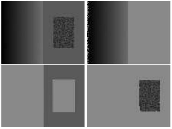
Figure 1: A synthetic image with three perceptually distinct regions, and the three largest regions found by our segmentation method (image 320 × 240 pixels; algorithm parameters σ = 0.8, k = 300, see Section 5 for an explanation of the parameters).
图 1:一幅具有三个明显感知区域的合成图像以及我们的分割方法发现的三个最大区域(图像320×240像素;算法参数σ=0.8,k=300,参数解释见第5节)
The organization of this paper is as follows. In the next Section we discuss some related work, including both classical formulations of segmentation and recent graph-based methods. In Section 3 we consider a particular graph-based formulation of the segmentation problem and define a pairwise region comparison predicate. Then in Section 4 we present an algorithm for efficiently segmenting an image using this predicate, and derive some global properties that it obeys even though it is a greedy algorithm. In Section 5 we show results for a number of images using the image grid to construct a graph-based representation of the image data. Then in Section 6 we illustrate the method using more general graphs, but where the number of edges is still linear in the number of pixels. Using this latter approach yields results that capture high-level scene properties such as extracting a flower bed as a single region, while still preserving fine detail in other portions of the image. In the Appendix we show that a straightforward generalization of the region comparison predicate presented in Section 3 makes the problem of finding a good segmentation NP-hard.
本文的组织结构如下。在下一节中,我们将讨论一些相关的工作,包括经典的分割公式和最新的基于图的方法。在第3节中,我们考虑了一个特殊的基于图的分割问题公式,并定义了一个成对区域比较谓词。然后,在第4节中,我们提出了一种使用该谓词有效分割图像的算法,并推导出它所遵循的一些全局属性,即使它是贪婪算法。在第5节中,我们展示了使用图像网格构建基于图的图像数据表示的多个图像的结果。然后在第6节中,我们用更一般的图来说明这个方法,但是在图中,边的数量仍然是像素数量的线性。使用后一种方法可以生成捕获高级场景属性的结果,例如将花坛提取为单个区域,同时在图像的其他部分保留精细细节。在附录中,我们证明了第3节中提出的区域比较谓词的一个简单概括使得找到一个好的分割变得NP-困难
相关工作
There is a large literature on segmentation and clustering, dating back over 30 years, with applications in many areas other than computer vision (cf. [9]). In this section we briefly consider some of the related work that is most relevant to our approach: early graph-based methods (e.g., [15, 19]), region merging techniques (e.g., [5, 11]), techniques based on mapping image pixels to some feature space (e.g., [3, 4]) and more recent formulations in terms of graph cuts (e.g., [14, 18]) and spectral methods (e.g., [16]).
关于分割和聚类的大量文献可以追溯到30多年前,在计算机视觉以外的许多领域都有应用(参见[9])。在本节中,我们简要地考虑了与我们的方法最相关的一些相关工作:早期基于图的方法(例如[15,19])、区域合并技术(例如[5,11])、基于将图像像素映射到某些特征空间的技术(例如[3,4])以及关于图形切割的更新公式(例如[14,18])和光谱方法(例如[16])
Graph-based image segmentation techniques generally represent the problem in terms of a graph
where each node corresponds to a pixel in the image, and the edges in connect certain pairs of neighboring pixels. A weight is associated with each edge based on some property of the pixels that it connects, such as their image intensities. Depending on the method, there may or may not be an edge connecting each pair of vertices. The earliest graph-based methods use fixed thresholds and local measures in computing a segmentation. The work of Zahn[19] presents a segmentation method based on the minimum spanning tree (MST) of the graph. This method has been applied both to point clustering and to image segmentation. For image segmentation the edge weights in the graph are based on the differences between pixel intensities, whereas for point clustering the weights are based on distances between points.
基于图的图像分割技术通常用图
The segmentation criterion in Zahn’s method is to break MST edges with large weights. The inadequacy of simply breaking large edges, however, is illustrated by the example in Figure 1. As mentioned in the introduction, differences between pixels within the high variability region can be larger than those between the ramp and the constant region. Thus, depending on the threshold, simply breaking large weight edges would either result in the high variability region being split into multiple regions, or would merge the ramp and the constant region together. The algorithm proposed by Urquhart [15] attempts to address this shortcoming by normalizing the weight of an edge using the smallest weight incident on the vertices touching that edge. When applied to image segmentation problems, however, this is not enough to provide a reasonable adaptive segmentation criterion. For example, many pixels in the high variability region of Figure 1 have some neighbor that is highly similar.
Zahn方法中的分割标准是用较大的权重分割MST边缘。然而,图1中的示例说明了简单地破坏大边缘的不足。正如在引言中提到的,高变率区域内像素之间的差异可能大于渐变和恒定区域之间的差异。因此,根据阈值的不同,简单地打破较大的权重边缘将导致高变率区域分割为多个区域,或者将斜坡和常量区域合并在一起。Urquhart[15]提出的算法试图通过使用与边缘接触的顶点上的最小权重来规范化边缘的权重来解决这一缺点。然而,当应用于图像分割问题时,这不足以提供一个合理的自适应分割标准。例如,图1的高可变性区域中的许多像素具有高度相似的邻居
Another early approach to image segmentation is that of splitting and merging regions according to how well each region fits some uniformity criterion (e.g., [5,11]). Generally these uniformity criteria obey a subset property, such that when a uniformity predicate
is true for some region then is also true for any . Usually such criteria are aimed at finding either uniform intensity or uniform gradient regions. No region uniformity criterion that has been proposed to date could be used to correctly segment the example in Figure 1, due to the high variation region. Either this region would be split into pieces, or it would be merged with the surrounding area.
另一种早期的图像分割方法是根据每个区域符合某种均匀性标准的程度来分割和合并区域(例如[5,11])。一般来说,这些一致性标准服从一个子集属性,当某个区域
A number of approaches to segmentation are based on finding compact clusters in some feature space (cf. [3, 9]). These approaches generally assume that the image is piecewise constant, because searching for pixels that are all close together in some feature space implicitly requires that the pixels be alike (e.g., similar color). A recent technique using feature space clustering [4] first transforms the data by smoothing it in a way that preserves boundaries between regions. This smoothing operation has the overall effect of bringing points in a cluster closer together. The method then finds clusters by dilating each point with a hypersphere of some fixed radius, and finding connected components of the dilated points. This technique for finding clusters does not require all the points in a cluster to lie within any fixed distance. The technique is actually closely related to the region comparison predicate that we introduce in Section 3.1, which can be viewed as an adaptive way of selecting an appropriate dilation radius. We return to this issue in Section 6.
许多分割方法都是基于在某些特征空间中找到紧密的聚类(参见[3,9])。这些方法通常假定图像是分段不变的,因为在某些特征空间中搜索所有相邻的像素隐含地要求像素相同(例如,相似的颜色)。最近的一种使用特征空间聚类的技术[4]首先通过平滑操作来转换数据以保留区域之间的边界。这种平滑操作的总体效果是使同一聚类中的点更靠近。然后,该方法通过用一个固定半径的超球体来扩张每个点,并找到扩张点的连接组件来找到聚类。这种寻找聚类的技术不需要聚类中位于固定距离内的所有点。该技术实际上与我们在第3.1节中介绍的区域比较谓词密切相关,它可以被视为选择适当扩张半径的一种自适应方法。我们将在第6节中讨论这个问题
Finally we briefly consider a class of segmentation methods based on finding minimum cuts in a graph, where the cut criterion is designed in order to minimize the similarity between pixels that are being split. Work by Wu and Leahy [18] introduced such a cut criterion, but it was biased toward finding small components. This bias was addressed with the normalized cut criterion developed by Shi and Malik [14], which takes into account self-similarity of regions. These cut-based approaches to segmentation capture non-local properties of the image, in contrast with the early graph-based methods. However, they provide only a characterization of each cut rather than of the final segmentation.
最后,我们简单地考虑了一类基于在图中找到最小分割集的分割方法,分割准则是最小化被分割像素之间的相似性。Wu和Leahy[18]的工作引入了这样一个切割标准,但它倾向于寻找小部件。利用Shi和Malik[14]提出的标准化切割标准解决了这种偏差,该标准考虑了区域的自相似性。与早期的基于图的分割方法相比,这些基于切割的分割方法捕获了图像的非局部特性。但是,它们只提供每个切割的特征,而不是最终分割的特征
The normalized cut criterion provides a significant advance over the previous work in [18], both from a theoretical and practical point of view (the resulting segmentations capture intuitively salient parts of an image). However, the normalized cut criterion also yields an NP-hard computational problem. While Shi and Malik develop approximation methods for computing the minimum normalized cut, the error in these approximations is not well understood. In practice these approximations are still fairly hard to compute, limiting the method to relatively small images or requiring computation times of several minutes. Recently Weiss [16] has shown how the eigenvector-based approximations developed by Shi and Malik relate to more standard spectral partitioning methods on graphs. However, all such methods are too slow for many practical applications.
从理论和实践的角度来看,归一化切割标准比[18]中之前的工作有了显著的进步(由此产生的分割可以直观地捕获图像的显著部分)。然而,归一化割准则也产生了一个NP-困难的计算问题。尽管Shi和Malik开发了计算最小归一化割集的近似方法,但这些近似中的误差还不太清楚。实际上,这些近似值仍然很难计算,将该方法限制在相对较小的图像上,或者需要几分钟的计算时间。最近,Weiss[16]已经展示了Shi和Malik开发的基于特征向量的近似与更标准的图上光谱划分方法的关系。然而,对于许多实际应用来说,所有这些方法都太慢了
An alternative to the graph cut approach is to look for cycles in a graph embedded in the image plane. For example in [10] the quality of each cycle is normalized in a way that is closely related to the normalized cuts approach.
另一种图切割方法是在嵌入图像平面的图中查找循环。例如,在[10]中每个循环的质量都以与标准化切割方法密切相关的方式进行标准化
基于图的分割
Graph-Based Segmentation
We take a graph-based approach to segmentation. Let
be an undirected graph with vertices , the set of elements to be segmented, and edges corresponding to pairs of neighboring vertices. Each edge has a corresponding weight , which is a non-negative measure of the dissimilarity between neighboring elements and . In the case of image segmentation, the elements in are pixels and the weight of an edge is some measure of the dissimilarity between the two pixels connected by that edge (e.g., the difference in intensity, color, motion, location or some other local attribute). In Sections 5 and 6 we consider particular edge sets and weight functions for image segmentation. However, the formulation here is independent of these definitions.
我们采用了一种基于图的分割方法。 设
In the graph-based approach, a segmentation
is a partition of into components such that each component (or region) corresponds to a connected component in a graph , where . In other words, any segmentation is induced by a subset of the edges in . There are different ways to measure the quality of a segmentation but in general we want the elements in a component to be similar, and elements in different components to be dissimilar. This means that edges between two vertices in the same component should have relatively low weights, and edges between vertices in different components should have higher weights.
在基于图的方法中,分割
成对区域比较渭词
Pairwise Region Comparison Predicate
In this section we define a predicate,
, for evaluating whether or not there is evidence for a boundary between two components in a segmentation (two regions of an image). This predicate is based on measuring the dissimilarity between elements along the boundary of the two components relative to a measure of the dissimilarity among neighboring elements within each of the two components. The resulting predicate compares the inter-component differences to the within component differences and is thereby adaptive with respect to the local characteristics of the data.
在本节中,我们定义一个谓词
We define the internal difference of a component
to be the largest weight in the minimum spanning tree of the component, . That is,
我们将分量
One intuition underlying this measure is that a given component C only remains connected when edges of weight at least Int(C) are considered.
这个度量的一个直觉是,给定的分量
We define the difference between two components
to be the minimum weight edge connecting the two components. That is,
我们将两个分量
If there is no edge connecting
and we let . This measure of difference could in principle be problematic, because it reflects only the smallest edge weight between two components. In practice we have found that the measure works quite well in spite of this apparent limitation. Moreover, changing the definition to use the median weight, or some other quantile, in order to make it more robust to outliers, makes the problem of finding a good segmentation NP-hard, as discussed in the Appendix. Thus a small change to the segmentation criterion vastly changes the difficulty of the problem.
如果
The region comparison predicate evaluates if there is evidence for a boundary between a pair or components by checking if the difference between the components,
, is large relative to the internal difference within at least one of the components, and . A threshold function is used to control the degree to which the difference between components must be larger than minimum internal difference. We define the pairwise comparison predicate as,
区域比较谓词通过检查分量间差异
where the minimum internal difference,
, is defined as,
其中最小内部差异
The threshold function
controls the degree to which the difference between two components must be greater than their internal differences in order for there to be evidence of a boundary between them (D to be true). For small components, is not a good estimate of the local characteristics of the data. In the extreme case, when , . Therefore, we use a threshold function based on the size of the component,
阈值函数
where
denotes the size of , and is some constant parameter. That is, for small components we require stronger evidence for a boundary. In practice sets a scale of observation, in that a larger causes a preference for larger components. Note, however, that is not a minimum component size. Smaller components are allowed when there is a sufficiently large difference between neighboring components.
其中
Any non-negative function of a single component can be used for
without changing the algorithmic results in Section 4. For instance, it is possible to have the segmentation method prefer components of certain shapes, by defining a which is large for components that do not fit some desired shape and small for ones that do. This would cause the segmentation algorithm to aggressively merge components that are not of the desired shape. Such a shape preference could be as weak as preferring components that are not long and thin (e.g., using a ratio of perimeter to area) or as strong as preferring components that match a particular shape model. Note that the result of this would not solely be components of the desired shape, however for any two neighboring components one of them would be of the desired shape.
在不改变第4节中算法结果的情况下,可以将单个分量的任何非负函数用于
算法及其性质
The Algorithm and Its Properties
In this section we describe and analyze an algorithm for producing a segmentation using the decision criterion
introduced above. We will show that a segmentation produced by this algorithm obeys the properties of being neither too coarse nor too fine, according to the following definitions.
在本节中,我们描述并分析了一种使用上述决策标准
Definition 1 A segmentation
is too fine if there is some pair of regions for which there is no evidence for a boundary between them.
定义 1 如果没有证据表明一些区域对
In order to define the complementary notion of what it means for a segmentation to be too coarse (to have too few components), we first introduce the notion of a refinement of a segmentation. Given two segmentations
and of the same base set, we say that is a refinement of when each component of is contained in (or equal to) some component of . In addition, we say that is a proper refinement of when .
为了定义分割过于粗糙(组件太少)意味着什么的互补概念,我们首先引入分割细化的概念。给定两个相同基集的分段
Definition 2 A segmentation
is too coarse when there exists a proper refinement of that is not too fine.
定义 2 当存在不太精细的适当细化时,分割
This captures the intuitive notion that if regions of a segmentation can be split and yield a segmentation where there is evidence for a boundary between all pairs of neighboring regions, then the initial segmentation has too few regions.
这捕捉到了一个直观的概念,即如果一次分割后的区域还可以被分割,并且再次分割后有证据表明所有相邻区域对之间存在边界,那么初始分割的区域太少
Two natural questions arise about segmentations that are neither too coarse nor too fine, namely whether or not one always exists, and if so whether or not it is unique. First we note that in general there can be more than one segmentation that is neither too coarse nor too fine, so such a segmentation is not unique. On the question of existence, there is always some segmentation that is both not too coarse and not too fine, as we now establish.
对于既不太粗也不太细的分割,会出现两个自然的问题,即是否总是存在一次分割操作,如果存在,是否是唯一一次分割(一次分割操作后就完成了)。首先,我们注意到,一般来说,可以有多次既不太粗也不太细的分割,因此这样的分割不是唯一的。在是否存在的问题上,总是存在一些既不太粗糙也不太精细的分割,正如我们现在所确定的
Property 1 For any (finite) graph
there exists some segmentation that is neither too coarse nor too fine.
属性一 对于任何(有限)图
It is easy to see why this property holds. Consider the segmentation where all the elements are in a single component. Clearly this segmentation is not too fine, because there is only one component. If the segmentation is also not too coarse we are done. Otherwise, by the definition of what it means to be too coarse there is a proper refinement that is not too fine. Pick one of those refinements and keep repeating this procedure until we obtain a segmentation that is not too coarse. The procedure can only go on for n−1 steps because whenever we pick a proper refinement we increase the number of components in the segmentation by at least one, and the finest segmentation we can get is the one where every element is in its own component.
很容易看出这个属性为什么会存在。考虑所有元素都在单个分量中的分割。显然,这种细分并不太精细,因为只有一个分量。如果分割也不太粗糙,我们就完成了。否则,通过太粗糙的定义可知需要有一个适当的细化。选择其中一个分量进行细化,并不断重复这个过程,直到我们得到一个不太粗糙的分割。这个过程最多进行n-1个步骤,因为每当我们选择分量进行适当的细化,我们都会将分割后的分量数量至少增加一个,我们可以得到的最好的分割是每个元素都在其自己的分量中
We now turn to the segmentation algorithm, which is closely related to Kruskal’s algorithm for constructing a minimum spanning tree of a graph (cf. [6]). It can be implemented to run in
time, where is the number of edges in the graph.
我们现在讨论的是分割算法,它与构建图的最小生成树的Kruskal算法密切相关(参见[6])。它可以实现在
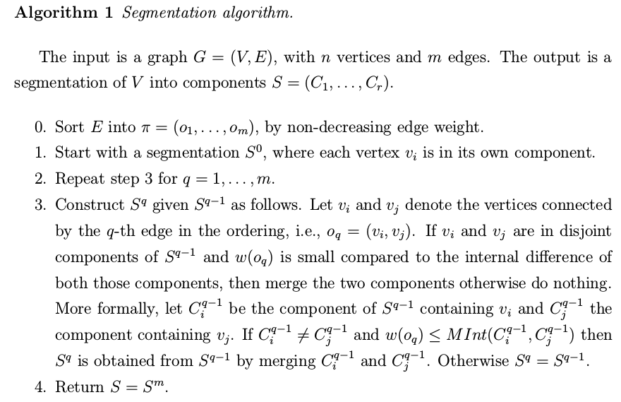
Algorithm 1 Segmentation algorithm
算法 1 分割算法
The input is a graph
, with vertices and edges. The output is a segmentation of into components .
输入是一个图
- Sort
into , by non-decreasing edge weight. - Start with a segmentation
, where each vertex is in its own component. - Repeat step
for . - Construct
given as follows. Let and denote the vertices connected by the -th edge in the ordering, i.e., . If and are in disjoint components of and is small compared to the internal difference of both those components, then merge the two components otherwise do nothing. More formally, let be the component of containing and the component containing . If and then is obtained from by merging and . Otherwise . - Return
- 按边权重递增排序边集
- 从分割
- 对于
- 给定
- 返回
We now establish that a segmentation
produced by Algorithm 1 obeys the global properties of being neither too fine nor too coarse when using the region comparison predicate defined in (3). That is, although the algorithm makes only greedy decisions it produces a segmentation that satisfies these global properties. Moreover, we show that any of the possible non-decreasing weight edge orderings that could be picked in Step 0 of the algorithm produce the same segmentation.
我们现在证明,当使用(3)中定义的区域比较渭词
Lemma 1 In Step
of the algorithm, when considering edge , if two distinct components are considered and not merged then one of these two components will be in the final segmentation. Let and denote the two components connected by edge when this edge is considered by the algorithm. Then either or , where is the component containing and is the component containing in the final segmentation .
引理 1 在算法的第
Proof. There are two cases that would result in a merge not happening. Say that it is due to
. Since edges are considered in non-decreasing weight order, , for all . Thus no additional merges will happen to this component, i.e., . The case for is analogous.
证明 只有两种情况会导致合并不发生。一是因为
Note that Lemma 1 implies that the edge causing the merge of two components is exactly the minimum weight edge between the components. Thus the edges causing merges are exactly the edges that would be selected by Kruskal’s algorithm for constructing the minimum spanning tree (MST) of each component.
注意,引理1说明导致两个分量合并的边恰好是分量之间的最小权重边。因此,导致分量合并的边也是Kruskal算法选择用于构造每个分量的最小生成树(MST)的边
Theorem 1 The segmentation
produced by Algorithm 1 is not too fine according to Definition 1, using the region comparison predicate defined in (3).
定理1 根据定义1,使用(3)中定义的区域比较谓词
Proof. By definition, in order for
to be too fine there is some pair of components for which does not hold. There must be at least one edge between such a pair of components that was considered in Step 3 and did not cause a merge. Let be the first such edge in the ordering. In this case the algorithm decided not to merge with which implies . By Lemma 1 we know that either or . Either way we see that implying holds for and , which is a contradiction.
证明 假设
Theorem 2 The segmentation
produced by Algorithm 1 is not too coarse according to Definition 2, using the region comparison predicate defined in (3).
定理 2 根据定义2,使用(3)中定义的区域比较谓词
Proof. In order for
to be too coarse there must be some proper refinement, , that is not too fine. Consider the minimum weight edge that is internal to a component but connects distinct components . Note that by the definition of refinement and .
证明 为了使
Since
is not too fine, either or . Without loss of generality, say the former is true. By construction any edge connecting to another sub-component of has weight at least as large as , which is in turn larger than the maximum weight edge in because . Thus the algorithm, which considers edges in non-decreasing weight order, must consider all the edges in before considering any edge from to other parts of . So the algorithm must have formed before forming , and in forming it must have merged with some other sub-component of . The weight of the edge that caused this merge must be least as large as . However, the algorithm would not have merged in this case because , which is a contradiction.
因为
Theorem 3 The segmentation produced by Algorithm 1 does not depend on which non-decreasing weight order of the edges is used.
定理 3 由算法1产生的分割集不依赖于边的权重递增顺序(应该指的是同一权重的不同边的顺序)
Proof. Any ordering can be changed into another one by only swapping adjacent elements. Thus it is sufficient to show that swapping the order of two adjacent edges of the same weight in the non-decreasing weight ordering does not change the result produced by Algorithm 1.
证明 任何顺序都可以通过交换相邻元素而更改为另一个顺序。因此,在非递减权重排序中交换同一权重的两个相邻边的顺序并不改变算法1产生的结果
Let
and be two edges of the same weight that are adjacent in some non-decreasing weight ordering. Clearly if when the algorithm considers the first of these two edges they connect disjoint pairs of components or exactly the same pair of components, then the order in which the two are considered does not matter. The only case we need to check is when is between two components and and is between one of these components, say , and some other component .
假定
Now we show that
causes a merge when considered after exactly when it would cause a merge if considered before . First, suppose that causes a merge when considered before . This implies . If were instead considered before , either would not cause a merge and trivially would still cause a merge, or would cause a merge in which case the new component would have . So we know which implies will still cause a merge. On the other hand, suppose that does not cause a merge when considered before . This implies . Then either , in which case this would still be true if were considered first (because does not touch ), or . In this second case, if were considered first it could not cause a merge since and so . Thus when considering after we still have and does not cause a merge.
假定
实施问题和运行时间
Implementation Issues and Running Time
Our implementation maintains the segmentation
using a disjoint-set forest with union by rank and path compression (cf. [6]). The running time of the algorithm can be factored into two parts. First in Step 0, it is necessary to sort the weights into non-decreasing order. For integer weights this can be done in linear time using counting sort, and in general it can be done in time using any one of several sorting methods.
我们的实现使用一个按秩和路径压缩联合的不相交森林来维护分割
Steps 1-3 of the algorithm take
time, where is the very slow-growing inverse Ackerman’s function. In order to check whether two vertices are in the same component we use set-find on each vertex, and in order to merge two components we use use set-union. Thus there are at most three disjoint-set operations per edge. The computation of can be done in constant time per edge if we know and the size of each component. Maintaining for a component can be done in constant time for each merge, as the maximum weight edge in the of a component is simply the edge causing the merge. This is because Lemma 1 implies that the edge causing the merge is the minimum weight edge between the two components being merged. The size of a component after a merge is simply the sum of the sizes of the two components being merged.
算法步骤1-3的时间复杂度为
网格图的结果
Results for Grid Graphs
First we consider the case of monochrome (intensity) images. Color images are handled as three separate monochrome images, as discussed below. As in other graph-based approaches to image segmentation (e.g., [14, 18, 19]) we define an undirected graph
, where each image pixel has a corresponding vertex . The edge set is constructed by connecting pairs of pixels that are neighbors in an 8-connected sense (any other local neighborhood could be used). This yields a graph where , so the running time of the segmentation algorithm is for image pixels. We use an edge weight function based on the absolute intensity difference between the pixels connected by an edge,
首先,我们考虑单色(强度)图像的情况。彩色图像被处理为三个单独的单色图像,如下所述。 与其他基于图的图像分割方法(例如[14,18,19])一样,我们定义了一个无向图
where
is the intensity of the pixel . In general we use a Gaussian filter to smooth the image slightly before computing the edge weights, in order to compensate for digitization artifacts. We always use a Gaussian with , which does not produce any visible change to the image but helps remove artifacts.
其中
For color images we run the algorithm three times, once for each of the red, green and blue color planes, and then intersect these three sets of components. Specifically, we put two neighboring pixels in the same component when they appear in the same component in all three of the color plane segmentations. Alternatively one could run the algorithm just once on a graph where the edge weights measure the distance between pixels in some color space, however experimentally we obtained better results by intersecting the segmentations for each color plane in the manner just described.
对于彩色图像,我们分别为红色、绿色和蓝色的颜色平面运行算法,然后交叉这三组分量。具体地说,当两个相邻像素在所有三个颜色平面分割中都属于同一分量时,我们将其最终放置在同一个分量中。或者,可以在一个图上运行该算法一次,其中边权重测量某些颜色空间中像素之间的距离,但是在实验上,我们通过按刚才描述的方式相交每个颜色平面的分割获得了更好的结果
There is one runtime parameter for the algorithm, which is the value of
that is used to compute the threshold function . Recall we use the function where is the number of elements in . Thus effectively sets a scale of observation, in that a larger causes a preference for larger components. We use two different parameter settings for the examples in this section (and throughout the paper), depending on the resolution of the image and the degree to which fine detail is important in the scene. For instance, in the images of the COIL database of objects we use . In the or larger images, such as the street scene and the baseball player, we use .
算法有一个运行时参数,即用于计算阈值函数
The first image in Figure 2 shows a street scene. Note that there is considerable variation in the grassy slope leading up to the fence. It is this kind of variability that our algorithm is designed to handle (recall the high variability region in the synthetic example in Figure 1). The second image shows the segmentation, where each region is assigned a random color. The six largest components found by the algorithm are: three of the grassy areas behind the fence, the grassy slope, the van, and the roadway. The missing part of the roadway at the lower left is a visibly distinct region in the color image from which this segmentation was computed (a spot due to an imaging artifact). Note that the van is also not uniform in color, due to specular reflections, but these are diffuse enough that they are treated as internal variation and incorporated into a single region.
图2中的第一个图像显示了一个街道场景。请注意,通往围栏的草坡有相当大的变化。我们的算法正是被设计来处理这种可变性(回想一下图1中合成示例中的高可变性区域)。第二幅图像显示了分割,每个区域被分配一个随机颜色。算法发现的六个最大的分量是:栅栏后面的三个草地区域、草地斜坡、货车和道路。左下角的道路缺失部分是彩色图像中一个明显不同的区域,从中可以计算出该分割(图像伪影造成的斑点)。请注意,由于镜面反射,面包车的颜色也不均匀,但这些面包车的漫反射程度足以将其视为内部变化并合并到单个区域中
The first image in Figure 3 shows two baseball players (from [14]). As in the previous example, there is a grassy region with considerable variation. The uniforms of the players also have substantial variation due to folds in the cloth. The second image shows the segmentation. The six largest components found by the algorithm are: the back wall, the Mets emblem, a large grassy region (including part of the wall under the top player), each of the two players’ uniforms, and a small grassy patch under the second player. The large grassy region includes part of the wall due to the relatively high variation in the region, and the fact that there is a long slow change in intensity (not strong evidence for a boundary) between the grass and the wall. This “boundary” is similar in magnitude to those within the player uniforms due to folds in the cloth.
图3中的第一张图片显示了两名棒球运动员(来自[14])。和前面的例子一样,有一个有相当大变化的长满草的区域。由于布料的褶皱,运动员的制服也有很大的变化。第二幅图像显示了分割。算法发现的六个最大的分量是:后墙、大都会会徽、一个大的草区(包括顶部球员下方的部分墙)、两名球员的制服,以及第二名球员下方的一个小草区。由于该区域的变化相对较大,且草与墙之间的强度变化缓慢(没有强有力的边界证据),因此大型草地区域包括墙的一部分。这个“边界”在数量上与球员制服内的边界相似,因为布料上有褶皱
Figure 4 shows the results of the algorithm for an image of an indoor scene, where both fine detail and larger structures are perceptually important. Note that the segmentation preserves small regions such as the name tags the people are wearing and things behind the windows, while creating single larger regions for high variability areas such as the air conditioning duct near the top of the image, the clothing and the furniture. This image also shows that sometimes small “boundary regions” are found, for example at the edge of the jacket or shirt. Such narrow regions occur because there is a one or two pixel wide area that is halfway between the two neighboring regions in color and intensity. This is common in any segmentation method based on grid graphs. Such regions can be eliminated if desired, by removing long thin regions whose color or intensity is close to the average of neighboring regions.
图4显示了一个室内场景图像的算法结果,在这个场景中,精细的细节和较大的结构在感知上都很重要。请注意,分割保留了小区域,如人们所戴的姓名标签和窗户后面的东西,同时为高变化区域创建了单个较大的区域,如靠近图像顶部的空调管道、衣服和家具。这张图片还显示了有时会发现一些小的“边界区域”,例如在夹克或衬衫的边缘。这种狭窄区域的出现是因为在颜色和强度上,两个相邻区域之间有一个或两个像素宽的区域。这在任何基于网格图的分割方法中都很常见。如果需要,可以通过去除颜色或强度接近相邻区域平均值的细长区域来消除这些区域
Figure 5 shows three simple objects from the Columbia COIL image database. Shown for each is the largest region found by our algorithm that is not part of the black background. Note that each of these objects has a substantial intensity gradient across the face of the object, yet the regions are correctly segmented. This illustrates another situation that the algorithm was designed to handle, slow changes in intensity due to lighting.
图5显示了哥伦比亚COIL图像数据库中的三个简单对象。显示的每个区域都是我们的算法发现的最大区域,不是黑色背景的一部分。请注意,这些对象的每个面都有一个很大的强度梯度,但是区域是正确分割的。这说明了另一种该算法设计处理的情况,即照明导致的亮度变化缓慢
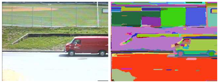
Figure 2: A street scene (
color image), and the segmentation results produced by our algorithm ( ).
图 2:街景(
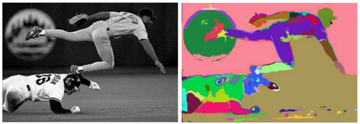
Figure 3: A baseball scene (
grey image), and the segmentation results produced by our algorithm ( ).
图 3:棒球场景(
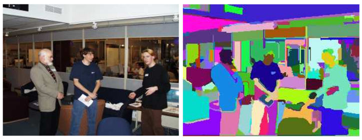
Figure 4: An indoor scene (image
, color), and the segmentation results produced by our algorithm ( ).
图 4:室内场景(
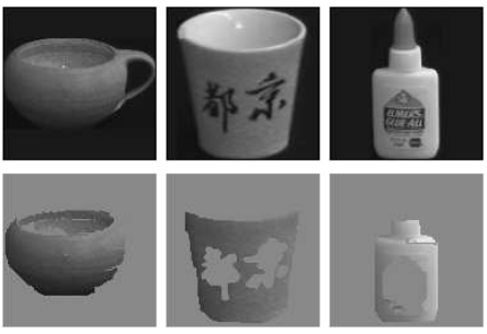
Figure 5: Three images from the COIL database, , and the largest non-background component found in each image (
color images; algorithm parameters ).
图 5:COIL数据集的3张图片,以及每张图片最大的非背景分量(
最近邻图的结果
Results for Nearest Neighbor Graphs
One common approach to image segmentation is based on mapping each pixel to a point in some feature space, and then finding clusters of similar points (e.g., [3, 4, 9]). In this section we investigate using the graph-based segmentation algorithm from Section 4 in order to find such clusters of similar points. In this case, the graph
has a vertex corresponding to each feature point (each pixel) and there is an edge connecting pairs of feature points and that are nearby in the feature space, rather than using neighboring pixels in the image grid. There are several possible ways of determining which feature points to connect by edges. We connect each point to a fixed number of nearest neighbors. Another possibility is to use all the neighbors within some fixed distance . In any event, it is desirable to avoid considering all pairs of feature points.
一种常见的图像分割方法是将每个像素映射到某些特征空间中的一个点,然后找到相似点的簇(例如[3,4,9])。 在本节中,我们使用第4节中基于图的分割算法,希望找到类似的点群。在这种情况下,图
The weight
of an edge is the distance between the two corresponding points in feature space. For the experiments shown here we map each pixel to the feature point , where is the location of the pixel in the image and is the color value of the pixel. We use the (Euclidean) distance between points as the edge weights, although other distance functions are possible.
边权重
The internal difference measure,
, has a relatively simple underlying intuition for points in feature space. It specifies the minimum radius of dilation necessary to connect the set of feature points contained in together into a single volume in feature space. Consider replacing each feature point by a ball with radius . From the definition of the it can be seen that the union of these balls will form one single connected volume only when . The difference between components, , also has a simple underlying intuition. It specifies the minimum radius of dilation necessary to connect at least one point of to a point of . Our segmentation technique is thus closely related to the work of [4], which similarly takes an approach to clustering based on dilating points in a parameter space (however they first use a novel transformation of the data that we do not perform, and then use a fixed dilation radius rather than the variable one that we use).
内部差异测量
Rather than constructing the complete graph, where all points are neighbors of one another, we find a small fixed number of neighbors for each point. This results in a graph with
edges for image pixels, and an overall running time of the segmentation method of time. There are many possible ways of picking a small fixed number of neighbors for each point. We use the ANN algorithm [1] to find the nearest neighbors for each point. This algorithm is quite fast in practice, given a 5-dimensional feature space with several hundred thousand points. The ANN method can also find approximate nearest neighbors, which runs more quickly than finding the actual nearest neighbors. For the examples reported here we use ten nearest neighbors of each pixel to generate the edges of the graph.
我们没有构建一个完整的图,其中所有点都是彼此的邻居,而是为每个点找到一个固定数量的邻居。结果得到了一个具有
One of the key differences from the previous section, where the image grid was used to define the graph, is that the nearest neighbors in feature space capture more spatially non-local properties of the image. In the grid-graph case, all of the neighbors in the graph are neighbors in the image. Here, points can be far apart in the image and still be among a handful of nearest neighbors (if their color is highly similar and intervening image pixels are of dissimilar color). For instance, this can result segmentations with regions that are disconnected in the image, which did not happen in the grid-graph case.
与上一节(使用图像网格定义图)的主要区别之一是,特征空间中最近邻捕获的图像具有更大的空间非局部属性。在网格图的情况下,图中的所有邻居都是图像中的邻居。在这里,点可以在图像中相距很远,并且仍然是特征空间中最近的邻居之一(如果它们的颜色非常相似,并且中间的图像像素的颜色不同)。例如,这可能会导致图像中断开的同一区域分割,而网格图中没有发生这种情况
Figure 6 shows a synthetic image from [12] and [8] and its segmentation, using
and with no smoothing ( ). In this example the spatially disconnected regions do not reflect interesting scene structures, but we will see examples below which do.
图6显示了来自[12]和[8]的合成图像及其分割,使用
For the remaining examples in this section, we use
and , as in the previous section. First, we note that the nearest neighbor graph produces similar results to the grid graph for images in which the perceptually salient regions are spatially connected. For instance, the street scene and baseball player scene considered in the previous section yield very similar segmentations using either the nearest neighbor graph or the grid graph, as can be seen by comparing the results in Figure 7 with those in Figure 2 and Figure 3.
对于本节中的其余示例,我们使用
Figure 8 shows two additional examples using the nearest neighbor graph. These results are not possible to achieve with the grid graph approach because certain interesting regions are not spatially connected. The first example shows a flower garden, where the red flowers are spatially disjoint in the foreground of the image, and then merge together in the background. Most of these flowers are merged into a single region, which would not be possible with the grid-graph method. The second example in Figure 8 shows the Eiffel tower at night. The bright yellow light forms a spatially disconnected region. These examples show that the segmentation method, coupled with the use of a nearest neighbor graph, can capture very high level properties of images, while preserving perceptually important region boundaries.
图8显示了使用最近邻图的另外两个示例。这些结果不可能使用网格图的方法实现,因为某些有趣的区域没有空间连接。 第一个例子显示了一个花园,在图像的前景中,红色的花在空间上是不相交的,但是在背景中合并在一起。这些花中的大多数被合并到一个单一的区域,这是使用网格图方法不可能实现的。图8中的第二个例子显示了晚上的埃菲尔铁塔。明亮的黄光形成一个空间上不相连的区域。这些实例表明,该分割方法结合最近邻图的使用,可以捕捉图像的高层次属性,同时保留感知上重要的区域边界
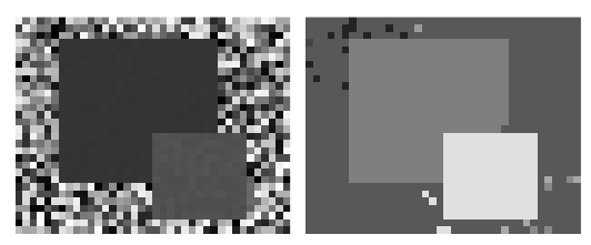
Figure 6: A synthetic image (
grey image) and the segmentation using the nearest neighbor graph ( ).
图 6:合成图像(
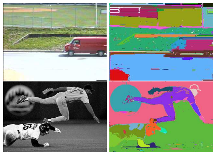
Figure 7: Segmentation of the street and baseball player scenes from the previous section, using the nearest neighbor graph rather than the grid graph (
).
图 7:使用最近邻图分割上一节使用的街景和棒球场景(
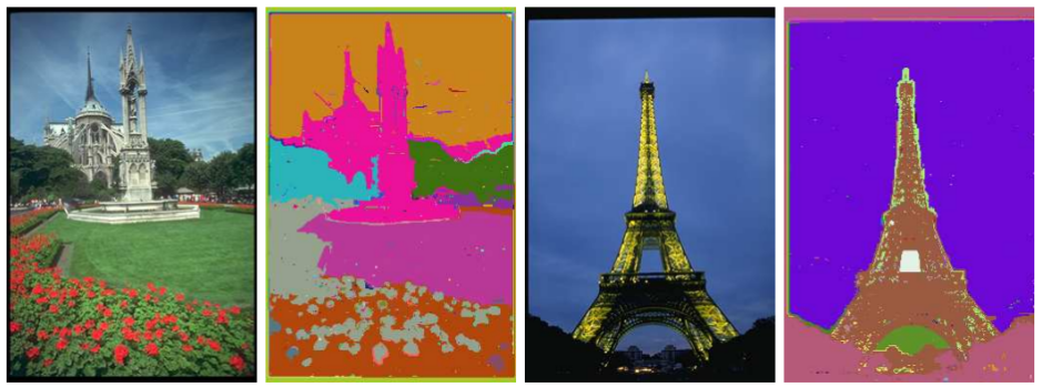
Figure 8: Segmentation using the nearest neighbor graph can capture spatially non-local regions (
).
图 8:使用最近邻图的分割(
总结和结论
Summary and Conclusions
In this paper we have introduced a new method for image segmentation based on pairwise region comparison. We have shown that the notions of a segmentation being too coarse or too fine can be defined in terms of a function which measures the evidence for a boundary between a pair of regions. Our segmentation algorithm makes simple greedy decisions, and yet produces segmentations that obey the global properties of being not too coarse and not too fine according to a particular region comparison function. The method runs in
time for graph edges and is also fast in practice, generally running in a fraction of a second.
本文介绍了一种基于成对区域比较的图像分割方法。我们已经证明,分割过粗或过细的概念可以用一个函数来定义,该函数测量一对区域之间边界的证据。我们的分割算法可以做出简单的贪婪决策,但根据特定的区域比较函数,可以产生符合不太粗糙和不太精细的全局属性的分割。该方法对
The pairwise region comparison predicate we use considers the minimum weight edge between two regions in measuring the difference between them. Thus our algorithm will merge two regions even if there is a single low weight edge between them. This is not as much of a problem as it might first appear, in part because this edge weight is compared only to the minimum spanning tree edges of each component. For instance, the examples considered in Sections 5 and 6 illustrate that the method finds segmentations that capture many perceptually important aspects of complex imagery. Nonetheless, one can envision measures that require more than a single cheap connection before deciding that there is no evidence for a boundary between two regions. One natural way of addressing this issue is to use a quantile rather than the minimum edge weight. However, in this case finding a segmentation that is neither too coarse nor too fine is an NP-hard problem (as shown in the Appendix). Our algorithm is unique, in that it is both highly efficient and yet captures non-local properties of images.
我们使用的成对区域比较谓词在测量两个区域之间的差异时考虑了两个区域之间的最小权重边。因此,我们的算法将合并两个区域,即使它们之间有一个单独的低权重边。这并不是第一次出现的问题,部分原因是边权重只与每个分量的最小生成树的边进行比较。例如,第5节和第6节中考虑的示例说明,该方法发现了捕捉复杂图像许多重要方面的分割。尽管如此,在决定两个区域之间没有边界的证据之前,我们可以设想需要一个以上连接的措施。解决这个问题的一种自然方法是使用分位数,而不是最小边权重。然而,在这种情况下,找到既不太粗糙也不太精细的分割是一个NP难题(如附录所示)。我们的算法是独一无二的,因为它既高效又能捕捉图像的非局部特性
We have illustrated our image segmentation algorithm with two different kinds of graphs. The first of these uses the image grid to define a local neighborhood between image pixels, and measures the difference in intensity (or color) between each pair of neighbors. The second of these maps the image pixels to points in a feature space that combines the
location and color value. Edges in the graph connect points that are close together in this feature space. The algorithm yields good results using both kinds of graphs, but the latter type of graph captures more perceptually global aspects of the image.
我们用两种不同的图说明了我们的图像分割算法。第一种方法使用图像网格定义图像像素之间的局部邻域,并测量每对邻域之间的强度(或颜色)差异。第二个将图像像素映射到特征空间中的点,该特征空间组合了
Image segmentation remains a challenging problem, however we are beginning to make substantial progress through the introduction of graph-based algorithms that both help refine our understanding of the problem and provide useful computational tools. The work reported here and the normalized cuts approach [14] are just a few illustrations of these recent advances.
图像分割仍然是一个具有挑战性的问题,但是我们开始通过引入基于图的算法取得实质性进展,这两种算法都有助于改进我们对问题的理解,并提供有用的计算工具。这里报告的工作和标准化切割方法[14]只是这些最新进展的几个例子
Gitalk 加载中 ...