从numpy到pytorch实现逻辑回归

逻辑回归常用于二元分类任务,其使用交叉熵损失进行梯度计算,实现步骤如下:

  1. 加载、打乱、标准化训练和测试数据
  2. 设计分类器、损失函数和梯度更新函数
  3. 用训练数据计算目标函数和精度
  4. 用训练数据计算损失函数和梯度,并更新梯度
  5. 重复3-4步,直到精度达到要求或达到指定迭代次数
  6. 用测试数据计算目标函数和精度

使用numpypytorch分别实现小批量梯度下降的2分类逻辑回归

关键参数

  • 批量大小:128
  • 迭代次数:50000
  • 学习步长:0.0001

测试数据

使用numeric类型的德国信用数据,其包含24个变量和一个2类标签 - german.data-numeric

numpy实现

1
2
3
4
5
6
7
8
9
10
11
12
13
14
15
16
17
18
19
20
21
22
23
24
25
26
27
28
29
30
31
32
33
34
35
36
37
38
39
40
41
42
43
44
45
46
47
48
49
50
51
52
53
54
55
56
57
58
59
60
61
62
63
64
65
66
67
68
69
70
71
72
73
74
75
76
77
78
79
80
81
82
83
84
85
86
87
88
89
90
91
92
93
94
95
96
97
98
99
100
101
102
103
104
105
106
107
108
109
110
111
112
113
114
115
116
117
118
119
120
121
122
123
124
125
126
127
128
129
130
131
132
133
134
135
136
137
138
139
140
141
142
143
144
145
146
147
148
149
150
import matplotlib.pyplot as plt
import numpy as np
import pandas as pd
from sklearn.model_selection import train_test_split
import warnings

warnings.filterwarnings('ignore')

data_path = '../data/german.data-numeric'


def load_data(tsize=0.8, shuffle=True):
data_list = pd.read_csv(data_path, header=None, sep='\s+')

data_array = data_list.values
height, width = data_array.shape[:2]
data_x = data_array[:, :(width - 1)]
data_y = data_array[:, (width - 1)]

x_train, x_test, y_train, y_test = train_test_split(data_x, data_y, train_size=tsize, test_size=(1 - tsize),
shuffle=shuffle)

y_train = np.atleast_2d(np.array(list(map(lambda x: 1 if x == 2 else 0, y_train)))).T
y_test = np.atleast_2d(np.array(list(map(lambda x: 1 if x == 2 else 0, y_test)))).T

return x_train, y_train, x_test, y_test


def init_weights(inputs):
"""
初始化权重,符合标准正态分布
"""
return np.atleast_2d(np.random.uniform(size=inputs)).T


def sigmoid(x):
return 1 / (1 + np.exp(-1 * x))


def logistic_regression(w, x):
"""
w大小为(n+1)x1
x大小为mx(n+1)
"""
z = x.dot(w)
return sigmoid(z)


def compute_loss(w, x, y, isBatch=True):
"""
w大小为(n+1)x1
x大小为mx(n+1)
y大小为mx1
"""
lr_value = logistic_regression(w, x)
if isBatch:
n = y.shape[0]
res = -1.0 / n * (y.T.dot(np.log(lr_value)) + (1 - y.T).dot(np.log(1 - lr_value)))
return res[0][0]
else:
res = -1.0 * (y * (np.log(lr_value)) + (1 - y) * (np.log(1 - lr_value)))
return res[0]


def compute_gradient(w, x, y, isBatch=True):
"""
梯度计算
"""
lr_value = logistic_regression(w, x)
if isBatch:
n = y.shape[0]
return 1.0 / n * x.T.dot(lr_value - y)
else:
return np.atleast_2d(1.0 * x.T * (lr_value - y)).T


def compute_predict_accuracy(predictions, y):
results = predictions > 0.5
res = len(list(filter(lambda x: x[0] == x[1], np.dstack((results, y))[:, 0]))) / len(results)
return res


def draw(res_list, title=None, xlabel=None):
if title is not None:
plt.title(title)
if xlabel is not None:
plt.xlabel(xlabel)
plt.plot(res_list)
plt.show()


if __name__ == '__main__':
# 加载训练和测试数据
# train_data, train_label, test_data, test_label = load_german_numeric(tsize=0.85, shuffle=False)
train_data, train_label, test_data, test_label = load_data()

# 根据训练数据计算均值和标准差
mu = np.mean(train_data, axis=0)
std = np.std(train_data, axis=0)

# 标准化训练和测试数据
train_data = (train_data - mu) / std
test_data = (test_data - mu) / std

# 添加偏置值
train_data = np.insert(train_data, 0, np.ones(train_data.shape[0]), axis=1)
test_data = np.insert(test_data, 0, np.ones(test_data.shape[0]), axis=1)

# 定义步长、权重和偏置值
lr = 0.0001
w = init_weights(train_data.shape[1])

# 计算目标函数/损失函数以及梯度更新
epoches = 50000
batch_size = 128
num = train_label.shape[0]

loss_list = []
accuracy_list = []
loss = 0
best_accuracy = 0
best_w = None
for i in range(epoches):
loss = 0
train_num = 0
for j in range(0, num, batch_size):
loss += compute_loss(w, train_data[j:j + batch_size], train_label[j:j + batch_size], isBatch=True)
train_num += 1
# 计算梯度
gradient = compute_gradient(w, train_data[j:j + batch_size], train_label[j:j + batch_size], isBatch=True)
# 权重更新
tempW = w - lr * gradient
w = tempW
# 计算损失值
loss_list.append(loss / train_num)

# 计算精度
accuracy = compute_predict_accuracy(logistic_regression(w, train_data), train_label)
accuracy_list.append(accuracy)

if accuracy > best_accuracy:
best_accuracy = accuracy
best_w = w.copy()

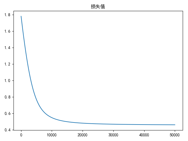
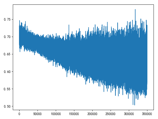
draw(loss_list, title='损失值')
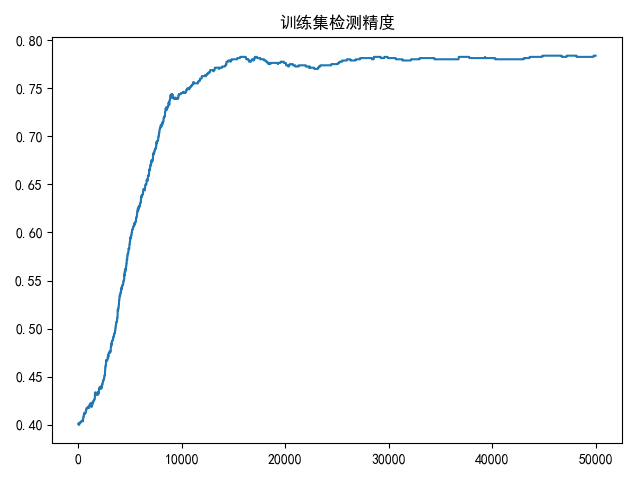
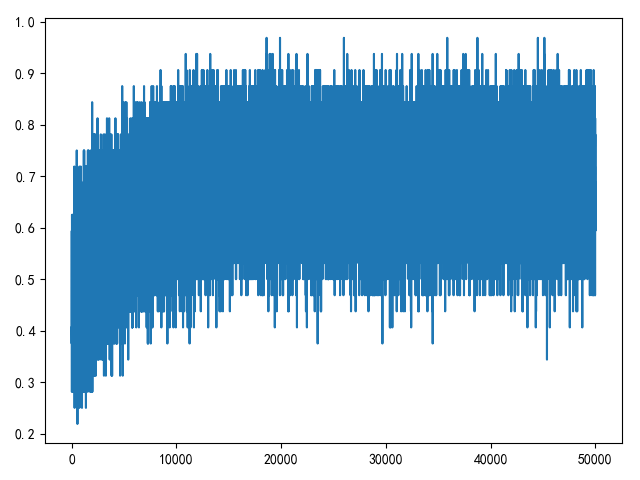
draw(accuracy_list, title='训练集检测精度')
print('train accuracy: %.3f' % (max(accuracy_list)))

test_accuracy = compute_predict_accuracy(logistic_regression(best_w, test_data), test_label)
print('test accuracy: %.3f' % (test_accuracy))

训练和测试精度:

1
2
train accuracy: 0.784
test accuracy: 0.765

训练损失图和精度图

pytorch实现

获取数据,转换成pytorch.Tensor数据格式,并进行数据标准化

1
2
3
4
5
6
7
8
9
10
11
12
13
14
15
16
17
18
19
20
21
22
23
24
def load_data(tsize=0.8, shuffle=True):
data_list = pd.read_csv(data_path, header=None, sep='\s+')

data_array = data_list.values
height, width = data_array.shape[:2]
data_x = data_array[:, :(width - 1)]
data_y = data_array[:, (width - 1)]

x_train, x_test, y_train, y_test = train_test_split(data_x, data_y, train_size=tsize, test_size=(1 - tsize),
shuffle=shuffle)

y_train = np.atleast_2d(np.array(list(map(lambda x: 1 if x == 2 else 0, y_train)))).T
y_test = np.atleast_2d(np.array(list(map(lambda x: 1 if x == 2 else 0, y_test)))).T

return torch.FloatTensor(x_train), torch.LongTensor(y_train), torch.FloatTensor(x_test), torch.LongTensor(y_test)

train_data, train_label, test_data, test_label = load_data(tsize=0.8, shuffle=True)

# 标准化数据
mu = torch.mean(train_data)
std = torch.std(train_data)

train_data = (train_data - mu) / std
test_data = (test_data - mu) / std

使用torch.utils.data.TensorDataSet加载数据和标签,使用torch.utils.data.DataLoader进行数据分片和打乱

1
2
3
batch_size = 16
data_ts = TensorDataset(train_data, train_label)
data_loader = DataLoader(data_ts, batch_size=batch_size, shuffle=True)

使用torch.nn.Linear进行线性运算,使用torch.nn.Sigmoid进行sigmoid运算

1
2
linear_model = nn.Linear(train_data.size()[1], 2)
sigmoid_model = nn.Sigmoid()

使用torch.nn.CrossEntropyLoss进行交叉熵损失计算,使用torch.optim.SGD进行小批量梯度下降

1
2
criterion = nn.CrossEntropyLoss()
optimizer = optim.SGD(linear_model.parameters(), lr=0.01)

完整代码如下:

1
2
3
4
5
6
7
8
9
10
11
12
13
14
15
16
17
18
19
20
21
22
23
24
25
26
27
28
29
30
31
32
33
34
35
36
37
38
39
40
41
42
43
44
45
46
47
48
49
50
51
52
53
54
55
56
57
58
59
60
61
62
63
64
65
66
67
68
69
70
71
72
73
74
75
76
77
78
79
80
81
82
83
84
85
86
87
88
89
90
91
92
93
94
95
96
97
98
99
100
101
102
103
104
105
106
import matplotlib.pyplot as plt
import pandas as pd
import numpy as np
from sklearn.model_selection import train_test_split
import torch
import torch.nn as nn
import torch.optim as optim
from torch.utils.data import TensorDataset
from torch.utils.data import DataLoader
import warnings

warnings.filterwarnings('ignore')

data_path = '../data/german.data-numeric'


def load_data(tsize=0.8, shuffle=True):
data_list = pd.read_csv(data_path, header=None, sep='\s+')

data_array = data_list.values
height, width = data_array.shape[:2]
data_x = data_array[:, :(width - 1)]
data_y = data_array[:, (width - 1)]

x_train, x_test, y_train, y_test = train_test_split(data_x, data_y, train_size=tsize, test_size=(1 - tsize),
shuffle=shuffle)

y_train = np.atleast_2d(np.array(list(map(lambda x: 1 if x == 2 else 0, y_train)))).T
y_test = np.atleast_2d(np.array(list(map(lambda x: 1 if x == 2 else 0, y_test)))).T

return torch.FloatTensor(x_train), torch.LongTensor(y_train), torch.FloatTensor(x_test), torch.LongTensor(y_test)


def compute_predict_accuracy(predictions, y):
results = torch.max(predictions, 1)[1]
res = len(list(filter(lambda x: x[0] == x[1], torch.t(torch.stack((results, y.squeeze())))))) / len(results)
return res


def draw(res_list):
plt.plot(res_list)
plt.show()


if __name__ == '__main__':
train_data, train_label, test_data, test_label = load_data(tsize=0.8, shuffle=True)

# 标准化数据
mu = torch.mean(train_data)
std = torch.std(train_data)

train_data = (train_data - mu) / std
test_data = (test_data - mu) / std

batch_size = 128
data_ts = TensorDataset(train_data, train_label)
data_loader = DataLoader(data_ts, batch_size=batch_size, shuffle=True)

# 设计分类器
linear_model = nn.Linear(train_data.size()[1], 2)
sigmoid_model = nn.Sigmoid()

# 损失函数
criterion = nn.CrossEntropyLoss()

# 优化器
optimizer = optim.SGD(linear_model.parameters(), lr=0.00001)

epoches = 50000
loss_list = []
accuracy_list = []
best_accuracy = 0
w = None
b = None
for i in range(epoches):
data = None
labels = None
outputs = None
for j, items in enumerate(data_loader, 0):
# 获取数据
data, labels = items
# 计算目标函数
outputs = sigmoid_model(linear_model(data))
# 计算损失值
loss = criterion(outputs, labels.squeeze().long())
# 保存损失值
loss_list.append(loss.item())
# 清空梯度
optimizer.zero_grad()
# 计算梯度
loss.backward()
# 更新梯度
optimizer.step()
# 计算精度
accuracy = compute_predict_accuracy(outputs, labels)
accuracy_list.append(accuracy)
if accuracy >= best_accuracy:
w, b = linear_model.weight, linear_model.bias
best_accuracy = accuracy

draw(loss_list)
draw(accuracy_list)
print('train accuracy: %.3f' % (max(accuracy_list)))

test_accuracy = compute_predict_accuracy(torch.sigmoid(torch.matmul(test_data, torch.t(w)) + b), test_label)
print('test accuracy: %.3f' % (test_accuracy))

训练和测试精度:

1
2
train accuracy: 1.000
test accuracy: 0.710

训练损失图和精度图

创建分类器类

可以创建分类器类来进行前向操作和预测(逻辑回归操作中仅线性操作需要权重计算,所以前向操作中可以仅执行线性回归,在预测操作中执行完整操作)

1
2
3
4
5
6
7
8
9
10
11
class LrModule(nn.Module):

def __init__(self, input_size):
super(LrModule, self).__init__()
self.fc = nn.Linear(input_size, 2)

def forward(self, inputs):
return F.sigmoid(self.fc(inputs))

def get_weights(self):
return self.fc.weight, self.fc.bias

实现如下:

1
2
3
4
5
6
7
8
9
10
11
12
13
14
15
16
17
18
19
    # 设计分类器
model = LrModule(train_data.size()[1])
...
...
for j, items in enumerate(data_loader, 0):
# 获取数据
data, labels = items
# 计算目标函数
outputs = model.forward(data)
...
...
# 计算精度
accuracy = compute_predict_accuracy(outputs, labels)
accuracy_list.append(accuracy)
if accuracy >= best_accuracy:
w, b = model.get_weights()
best_accuracy = accuracy
...
...

训练和测试精度:

1
2
train accuracy: 0.969
test accuracy: 0.720

训练损失图和精度图

小结

pytorch使用到的类库如下所示

相关阅读