线性回归

发表于 2019-04-09 更新于 2021-07-09 分类于机器学习/machine learning 阅读次数：

本文字数： 7.5k 阅读时长 ≈ 14 分钟

主要内容如下：

回归和分类的区别
线性回归
最小二乘法
梯度下降法

回归和分类

回归和分类一样，都是对变量进行预测

回归是对连续型变量进行预测，回归预测建模是指建立输入变量X映射到连续输出变量Y的映射函数f

分类是对离散型或连续型变量进行预测，分类预测建模是指建立输入变量X映射到离散输出变量Y的映射函数f

比如，预测天气温度是回归问题，预测天气是下雨还是晴天就是分类问题

线性回归

线性回归（linear regression）是以线性模型来建模自变量和因变量之间关系的方法

\[ y=h(x;\theta) \]

其中\(x\)是自变量，\(y\)是因变量，\(\theta\)是模型参数

如果自变量\(x\)只有一个，那么这种问题称为单变量线性回归（或称为一元线性回归）；如果自变量\(x\)表示多个，那么成为多变量线性回归（或称为多元线性回归）

单变量线性回归

单变量线性问题可转换为求解二维平面上的直线问题

模型计算公式如下：

\[ y=w_{1}x+w_{0} \]

参数集合\(\theta = \left \{ w_{0},w_{1} \right \}\)

在学习过程中，需要判断参数\(w_{0}\)和\(w_{1}\)是否满足要求，即是否和所有数据点接近。使用均方误差（mean square error，简称MSE）来评估预测值和实际数据点的接近程度，模型评估公式如下：

\[ J(w_{0},w_{1})=\frac{1}{N}\sum_{i=1}^{N}(h(x_{i};\theta) - y_{i})^{2} \]

其中\(y_{i}\)表示真实数据，\(h\)表示估计值，\(J\)表示损失值

多变量线性回归

多变量线性回归计算公式如下：

\[ \left\{\begin{matrix} y_{1}=w_{0}+w_{1}\cdot x_{11}+...+w_{n}\cdot x_{1n}\\ y_{2}=w_{0}+w_{1}\cdot x_{21}+...+w_{n}\cdot x_{2n}\\ ...\\ y_{m}=w_{0}+w_{1}\cdot x_{m1}+...+w_{n}\cdot x_{mn} \end{matrix}\right. \]

参数\(m\)表示有\(m\)个等式，参数\(n\)表示每一组变量有\(n\)个参数。设\(x_{0}=1\)，计算公式如下：

\[ \left\{\begin{matrix} y_{1}=w_{0}\cdot x_{10}+w_{1}\cdot x_{11}+...+w_{n}\cdot x_{1n}\\ y_{2}=w_{0}\cdot x_{20}+w_{1}\cdot x_{21}+...+w_{n}\cdot x_{2n}\\ ...\\ y_{m}=w_{0}\cdot x_{m0}+w_{1}\cdot x_{m1}+...+w_{n}\cdot x_{mn} \end{matrix}\right. \]

此时每组参数个数增加为\(n+1\)，其向量化公式如下：

\[ Y=X\cdot W \]

其中

\[ Y_{m\times 1}=\begin{bmatrix} y_{1}\\ y_{2}\\ ...\\ y_{m} \end{bmatrix} \]

\[ X_{m\times (n+1)}=\begin{bmatrix} x_{10} & x_{11} & ... & x_{1n}\\ x_{20} & x_{21} & ... & x_{2n}\\ ... & ... & ... & ...\\ x_{m0} & x_{m1} & ... & x_{mn} \end{bmatrix} =\begin{bmatrix} 1 & x_{11} & ... & x_{1n}\\ 1 & x_{21} & ... & x_{2n}\\ ... & ... & ... & ...\\ 1 & x_{m1} & ... & x_{mn} \end{bmatrix} \]

\[ W_{(n+1)\times 1}= \begin{bmatrix} w_{0} \\ w_{1} \\ ... \\ w_{n} \end{bmatrix} \]

同样使用均方误差作为损失函数

\[ J(W)=\frac{1}{N}\sum_{i=1}^{N}(h(x_{i};W) - y_{i})^{2} \]

最小二乘法

利用最小二乘法（least square method）计算线性回归问题的参数，它通过最小化误差的平方和来求取目标函数的最优值，这样进一步转换为求取损失函数\(J\)的最小值，当\(J\)得到最小值时，参数偏导数一定为0

\[ loss=N*J=\sum_{i=1}^{N}(h(x_{i}:\theta) - y_{i})^{2} \]

有两种方式进行最小二乘法的计算，使用几何方式计算单变量线性回归问题，使用矩阵方式计算多变量线性回归问题

几何计算

当\(J\)得到最小值时，\(w_{0}\)和\(w_{1}\)的偏导数一定为0，所以参数\(w_{0}\)和\(w_{1}\)的计算公式如下：

\[ \frac{\varphi J}{\varphi w_{0}} =\frac{\varphi }{\varphi w_{0}}\frac{1}{N} \sum_{i=1}^{N}(h(x_{i})-y_{i})^{2} =\frac{\varphi }{\varphi w_{0}}\frac{1}{N} \sum_{i=1}^{N}(w_{0}+w_{1}\cdot x_{i}-y_{i})^{2} \] \[ =\frac{2}{N} \sum_{i=1}^{N}(w_{0}+w_{1}\cdot x_{i}-y_{i}) =2\cdot w_{0}+\frac{2}{N} \sum_{i=1}^{N}(w_{1}\cdot x_{i}-y_{i}) \]

\[ \frac{\varphi J}{\varphi w_{0}}=0 \Rightarrow w_{0}=-\frac{1}{N}\sum_{i=1}^{N}(w_{1}\cdot x_{i}-y_{i}) =\frac{1}{N}(\sum_{i=1}^{N}y_{i}-\sum_{i=1}^{N}w_{1}\cdot x_{i}) =\bar{y}-w_{1}\cdot \bar{x} \]

\[ \frac{\varphi J}{\varphi w_{1}} =\frac{\varphi }{\varphi w_{1}}\frac{1}{N} \sum_{i=1}^{N}(h(x_{i})-y_{i})^{2} =\frac{\varphi }{\varphi w_{1}}\frac{1}{N} \sum_{i=1}^{N}(w_{0}+w_{1}\cdot x_{i}-y_{i})^{2} \] \[ =\frac{2}{N} \sum_{i=1}^{N}(w_{0}+w_{1}\cdot x_{i}-y_{i})\cdot x_{i} =\frac{2\cdot w_{0}}{N}\sum_{i=1}^{N}x_{i}+\frac{2\cdot w_{1}}{N}\sum_{i=1}^{N}x_{i}\cdot x_{i}-\frac{2}{N}\sum_{i=1}^{N}x_{i}\cdot y_{i} \] \[ =2\cdot w_{0}\cdot \bar{x}+2\cdot w_{1}\cdot \bar{x^{2}}-2\cdot \bar{x\cdot y} \]

\[ \frac{\varphi J}{\varphi w_{1}}=0, w_{0}=\bar{y}-w_{1}\cdot \bar{x} \Rightarrow \bar{x}\cdot \bar{y}-w_{1}\cdot \bar{x}^{2}+w_{1}\cdot \bar{x^{2}}-\bar{x\cdot y}=0 \Rightarrow w_{1}=\frac{\bar{x\cdot y} - \bar{x}\cdot \bar{y}}{\bar{x^{2}}-\bar{x}^{2}} \]

最终得到的\(w_{0}\)和\(w_{1}\)的计算公式如下：

\[ w_{0}=\bar{y}-w_{1}\cdot \bar{x} \]

\[ w_{1}=\frac{\bar{x\cdot y} - \bar{x}\cdot \bar{y}}{\bar{x^{2}}-\bar{x}^{2}} \]

参数\(\bar{y}\)表示真实结果的均值
参数\(\bar{x}\)表示输入变量的均值
参数\(\bar{x\cdot y}\)表示输入变量和真实结果的乘积的均值
其他变量以此类推

矩阵计算

基本矩阵运算如下：

\[ (X\pm Y)^T = X^T\pm Y^T \]

\[ (X\cdot Y)^{T}=Y^{T}\cdot X^{T} \]

\[ (A^T)^T=A \]

\[ \left | A^{T} \right |=\left | A \right | \]

矩阵求导如下：

\[ \frac{\varphi (\theta ^{T}\cdot X)}{\varphi \theta}=X \]

\[ \frac{\varphi (X^{T}\cdot \theta )}{\varphi \theta}=X \]

\[ \frac{\varphi (\theta ^{T}\cdot \theta )}{\varphi \theta}=\theta \]

\[ \frac{\varphi (\theta ^{T}\cdot C\cdot \theta )}{\varphi \theta}=2\cdot C\cdot \theta \]

对多变量线性线性回归问题进行计算，

\[ J(W) =\frac{1}{N}\cdot \sum_{i=1}^{N}(h(x_{i};W)-y_{i})^2 =\frac{1}{N}(X\cdot W-Y)^{T}\cdot (X\cdot W -Y) \] \[ =\frac{1}{N}((X\cdot W)^T-Y^T)\cdot (X\cdot W-Y)) =\frac{1}{N}(W^T\cdot X^T-Y^T)\cdot (X\cdot W-Y)) \] \[ =\frac{1}{N}(W^T\cdot X^{T}\cdot X\cdot W-W^T\cdot X^{T}\cdot Y-Y^{T}\cdot X\cdot W+Y^{T}\cdot Y) \]

其中，\(W^T\cdot X^{T}\cdot Y\)是\(Y^{T}\cdot X\cdot W\)的转置，计算结果均为\(1\times 1\)的标量，所以大小相等，上式计算如下：

\[ J(W)=\frac{1}{N}(W^T\cdot X^{T}\cdot X\cdot W-2\cdot W^T\cdot X^{T}\cdot Y+Y^{T}\cdot Y) \]

求解\(\frac{\varphi J(W)}{\varphi W}=0\)

\[ \frac{\varphi J(W)}{\varphi W}=\frac{1}{N}\cdot X^{T}\cdot X\cdot W-\frac{1}{N}\cdot X^{T}\cdot Y=0 \]

\[ \Rightarrow X^{T}\cdot X\cdot W=X^{T}\cdot Y \]

\[ \Rightarrow W=(X^{T}\cdot X)^{-1}\cdot X^{T}\cdot Y \]

\(X^{T}\cdot X\)必须是非奇异矩阵，满足\(\left | X^{T}\cdot X \right |\neq 0\)，才能保证可逆

对于矩阵的秩，有以下定理

对于\(n\)阶矩阵\(A\)，当且仅当\(\left | A \right | \neq 0\)时，\(R(A_{n})=n\)，称\(A\)为满秩矩阵
\(R(A^T)=R(A)\)
\(R(AB)\leq min \left \{ R(A), R(B)\right \}\)
设\(A\)为\(m\times n\)矩阵，则\(0\leq (A)\leq min \left \{ m,n \right \}\)

所以矩阵\(X\)的秩\(R(X)\)需要为\(n+1\)（通常样本数量\(m\)大于变量数量\(n+1\)）时，才能保证能够使用最小二乘法的矩阵方式求解线性回归问题

示例

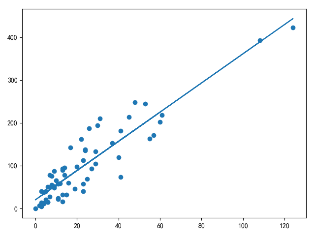
单边量线性回归测试数据参考[线性回归最小二乘法和梯度下降法]的瑞典汽车保险数据集

多变量线性回归测试数据参考coursera的ex1data2.txt

# -*- coding: utf-8 -*-

# @Time    : 19-4-16 上午10:04
# @Author  : zj

"""
最小二乘法计算线性回归问题
"""

from mpl_toolkits.mplot3d import Axes3D
import matplotlib.pyplot as plt
import numpy as np


def load_sweden_data():
    """
    加载单变量数据
    """
    path = '../data/sweden.txt'
    res = None
    with open(path, 'r') as f:
        line = f.readline()
        res = np.array(line.strip().split(' ')).reshape((-1, 2))
        # print(res)
    x = []
    y = []
    for i, item in enumerate(res, 0):
        item[1] = str(item[1]).replace(',', '.')
        # print('%d %.3f' % (int(item[0]), float(item[1])))
        x.append(int(item[0]))
        y.append(float(item[1]))
    return np.array(x), np.array(y)


def load_ex1_multi_data():
    """
    加载多变量数据
    """
    path = '../data/coursera2.txt'
    datas = []
    with open(path, 'r') as f:
        lines = f.readlines()
        for line in lines:
            datas.append(line.strip().split(','))
    data_arr = np.array(datas)
    data_arr = data_arr.astype(np.float)

    X = data_arr[:, :2]
    Y = data_arr[:, 2]
    return X, Y


def least_square_loss_v1(x, y):
    """
    最小二乘法，几何运算
    """
    X = np.array(x)
    Y = np.array(y)
    muX = np.mean(X)
    muY = np.mean(Y)
    muXY = np.mean(X * Y)
    muXX = np.mean(X * X)

    w1 = (muXY - muX * muY) / (muXX - muX ** 2)
    w0 = muY - w1 * muX
    return w0, w1


def least_square_loss_v2(x, y):
    """
    最小二乘法，矩阵运算
    """
    extend_x = np.insert(x, 0, values=np.ones(x.shape[0]), axis=1)
    w = np.linalg.inv(extend_x.T.dot(extend_x)).dot(extend_x.T).dot(y)
    return w


def compute_single_variable_linear_regression():
    x, y = load_sweden_data()
    w0, w1 = least_square_loss_v1(x, y)

    y2 = w1 * x + w0

    plt.scatter(x, y)
    plt.plot(x, y2)

    plt.show()


def compute_multi_variable_linear_regression():
    x, y = load_ex1_multi_data()
    # 计算权重
    w = least_square_loss_v2(x, y)
    print(w)


if __name__ == '__main__':
    # compute_single_variable_linear_regression()
    compute_multi_variable_linear_regression()

适用范围

最小二乘法直接进行计算就能求出解，操作简洁，最适用于计算单变量线性回归问题

而对于多变量线性回归问题，使用最小二乘法计算需要考虑计算效率，因为\(X^T\cdot X\)的逆矩阵计算代价很大，同时需要考虑可逆问题，所以更推荐梯度下降算法来解决多变量线性回归问题

小结

本文学习了线性回归模型，利用最小二乘法（最小化误差的平方和）实现单边量/多变量线性数据的训练和预测

在训练过程中，线性回归模型使用线性映射进行前向计算，利用均方误差方法进行损失值的计算

对于单变量线性回归问题，适用于最小二乘法的几何计算
对于多变量线性回归问题，如果变量维数不大同时满足\(\left | X^{T}\cdot X \right |\neq 0\)且\(R(X) = n+1\)的情况，使用最小二乘法的矩阵计算；否则，利用梯度下降方式进行权重更新

线性回归模型更适用于回归问题，可以使用逻辑回归模型进行分类

大海

线性回归

回归和分类

线性回归

单变量线性回归

多变量线性回归

最小二乘法

几何计算

矩阵计算

示例

适用范围

小结

相关阅读